Design and Analysis of Some Third Order
Explicit Almost Runge-Kutta Methods
Abdulrahman Ndanusa, Khadeejah James Audu
Department of Mathematics, Federal University of Technology, Minna, Nigeria
Received 19 December 2015; accepted 11 January 2016; published 14 January 2016 Copyright © 2016 by authors and Scientific Research Publishing Inc.
This work is licensed under the Creative Commons Attribution International License (CC BY). http://creativecommons.org/licenses/by/4.0/
Abstract
In this paper, we propose two new explicit Almost Runge-Kutta (ARK) methods, ARK3 (a three stage third order method, i.e., s = p = 3) and ARK34 (a four-stage third-order method, i.e., s = 4, p = 3), for the numerical solution of initial value problems (IVPs). The methods are derived through the application of order and stability conditions normally associated with Runge-Kutta methods; the derived methods are further tested for consistency and stability, a necessary requirement for convergence of any numerical scheme; they are shown to satisfy the criteria for both consistency and stability; hence their convergence is guaranteed. Numerical experiments carried out further justified the efficiency of the methods.
Keywords
Almost Runge-Kutta, Stability, Consistency, Convergence, Order Conditions, Rooted Trees
1. Introduction
According to [1] the s-stage Runge-Kutta method for solving the initial value problem
(
,)
,( )
0 0,y′ = f x y y x = y (1) is defined by
1
1 , s
n n i i
i
y+ y h b k
=
= +
∑
(2) where1
, , 1, 2, , ,
s
i n i n ij j
j
k f x c h y h a k i s
=
= + + =
and
1
1, 2, 3, ,
, .
s
i ij
j
c a i s
=
=
∑
= (4)Alternative forms of the above equations are:
(
)
1
1
, ,
s
n n i n i i
i
y+ y h b f x c h Y
=
= +
∑
+ (5)where
(
)
1
, , 1, , .
s
i n ij n j j
j
Y y h a f x c h Y i s
=
= +
∑
+ = (6)The two forms of Equations (2) and (5) are equivalent by making the interpretation
(
,)
, 1, ,i n i i
k = f x +c h Y i= s (7) where Yi is the inner stages that tend to estimate the solutions at some points; s is the number of stages and ci
is the points where the function f is computed for a step. ARK methods are a special class of RK methods that arose out of the quest to develop efficient and accurate methods that have advantages over the traditional me-thods by retaining the simple stability function of RK meme-thods, allowing minimal information to be passed be-tween steps and adjusting stepsize easily. Since the introduction of ARK methods in by [2], other researchers who have made their input toward the development of this method include [3]-[7].
2. Materials and Methods
2.1. Method ARK3 (
s
=
p
= 3)
The general third order three stages Almost Runge-Kutta scheme is of the form: 2
1 1
2
21 2 21 2 21 1
1 2 0
1 2 0
1 2 3 0
1
0 0 0 1
2 1
0 0 1
2
.
0 1 0
0 1 0
0 0 1 0 0 0
0 0
c c
a c a c a c
A U
b b b
B V
b b b
β β β β
− −
=
(8)
We represent the abscissa vector c=
[
c c1, 2,1 ,]
T bT =[
b b1, 2, 0 ,]
βT=[
β β β1, 2, 3]
.The order conditions for order three ARK schemes are derived through the standard rooted tree approach used for Runge-Kutta methods [8].
T
0 0 1 2
T
1 1 2 2
T 2 2 2
1 1 2 2
1 1
1 1
.
2 2
1 1
3 3
b b e b b b
b c b c b c
b c b c b c
+ = + + =
= ⇒ + =
= + =
(9)
The conditions of Runge-Kutta stability for 3rd order, 3 stages are:
(
)
T T
3 3 3
I A e
3 1
2 6
(
)
(
)
3 3 1
3 2 3 2exp c
exp
β
β β
− = −
− (12)
where
( )
2 3
1
2 3! !
n
n
x x x
exp x x
n
= + + + + + .
Acquiring order 2 estimation with respect to 2nd scaled derivative for the 3rd outgoing solution, we need: T
0 0. e
β +β = (13) T
1. c
β = (14a) From Equation (12) we have,
2 3
3 3 3
1
2
3 3 3
1 1
2 1
2 6
. 1
1
2
c
β β β
β β β
− + −
= −
− +
(14b)
Solving Equation (9) we obtain
(
2)
11 2 1
3 2
. 6
c b
c c c
− =
− (15)
(
1)
22 2 1
3 2
. 6
c b
c c c
− = −
− (16)
1 2 1 2
0
1 2
6 3 3 2
. 6
c c c c
b
c c
− − +
= (17)
And from Equation (11), we obtain
(
)
21
2 1 3 1
1 .
3 2
a
b c β c
=
+ (18)
Evaluating both sides of Equation (10) we obtain
(
3 2 2)
(
)
1 a b21 2 3 b1 3, 2 b2 3, 3 0, 0, 3 .
β − β + β β + β β = β (19) This implies that
3 2
1 21 2 3 1 3 2
2 2 3
3 3
0
0 .
a b b
b
β β β
β β
β β
− + =
+ =
=
(20)
Thus Equation (13) becomes
0 1 2 3.
β = − −β β −β (21)
Two free parameters, β3 and c2 are required for an order three scheme. Thus T 8 1, ,1 15 2
c =
; and after
8 32
0 0 0 1
15 225
25 313 4
0 0 1
576 576 27
75 5
4 0 1 0
.
16 16
75 5
4 0 1 0
16 16
0 0 1 0 0 0
75 3
36 3 0 0
2 2
A U
B V
−
−
=
−
− −
(22)
2.2. Method ARK34 (
s
= 4,
p
= 3)
The third order four stages scheme has the general form:
2
1 1
2
21 2 21 2 21 1
2
31 32 3 31 32 3 31 1 31 2
1 2 3 0
1 2 3 4 0
1 2 3 4 0
1
0 0 0 0 1
2 1
0 0 0 1
2 1
0 0 1 .
2
0 1 0
1 0
0 0 0 1 0 0 0
0 0
c c
a c a c a c
A U
a a c a a c a c a c
B V
b b b b
b b b b b
β β β β β
− −
− − − −
=
(23)
Its stability function is expressed as
( )
2 3 41 .
2! 3!
z z
R z = + +z + +Kz (24)
The order conditions are derived using the standard rooted tree approach used for Runge-Kutta methods [8]. T 1
. 2
b c= (25)
T 2 1 . 3
b c = (26) T
0 1 .
b = −b e (27) T
0 e
β = −β (28)
(
)
(
)
T 2
4 4e I A I A 4 A .
β +θ = + ∅ +β θ (29)
3 2
4 1 3 4 4 1 1
1 1
1 1 .
2 2 2! 3!
K β θαc −α = + β c +α +α +α
(30)
The αi values are obtained by expanding
(
4)
2 0 4
1
. 1
i i i
z
z
z z
β
α β θ
∞
=
+ ∅ − =
+ ∅ +
∑
(31)(
)
6(
)
(
)
T 2 T 2
4 4
1
.
2b Ac K b A c K
β − = β − ∅ −
(33)
There is also the additional condition
T 3
b c =L (34)
1, 2, 3, 4, ,
c c c β ∅θ and L will be assumed to be the free parameters, where 1 4
L− is the error coefficient com-parable to the bushy tree. From Equations (25)-(27) together with Equation (34) we have
1 1 2 2 3 3
2 2 2
1 1 2 2 3 3
3 3 3
1 1 2 2 3 3
0 1 2 3
1 2 1
. 3
1
b c b c b c
b c b c b c
b c b c b c L
b b b b
+ + =
+ + =
+ + =
+ + + =
(35)
Thus
(
2 3)(
2)
3 13 1 2 1 1
3 6 2 2
. 6
c c L c c
b
c c c c c
+ − −
=
− − (36)
(
)(
)
1 3 1 3
2
2 2 1 3 2 6 2 2
. 6
Bc c L c c b
c c c c c
+ −
= −
− − (37)
(
1 2 1 2)
3 2
3 1 2 1 3 2 3 3
3 6 2 2
. 6
c c L c c b
c c c c c c c c
− −
=
− − + (38)
1 2 3 1 2 1 3 2 3 1 2 3 0
1 2 3
6 3 3 3 6 2 2 2
1
. 6
c c c c c c c c c L c c c
b
c c c
− + + + + − − −
= −
(39)
From Equation (30) we obtain
3 2
4 1 1
4 1 3 4
1
1 1
2 2! 3!
. 1
2
c K
c
α α
β α
β θα α
+ + + +
=
−
(40)
Evaluating the stability matrix of a four stage third order method, we arrive at
(
3)
Tr BA U =K. (41) where Tr is the trace of a matrix and
(
)
(
)
(
)
3 T 3 T 3 T 2
3 3 T 3 T 3 T 2
3 T 3 T 3 T 2
1 2 1
. 2
1 2
s s s
A b e A c Ae A b c Ac
BA U A e A e c Ae A e c Ac
A e A c Ae A c Ac
β
β β β
− −
= − −
− −
(42)
(
3)
T 3 T 3(
)
T 3 1 2Tr .
2 s
BA U =b A e+e A c−Ae +β A c −Ac
(43)
(
)
T 3 T 3 T 3 1 2
. 2
s
b A e+e A c−Ae +β A c −Ac=K
(44)
And it follows that:
T 2 1 T 3 2 T 4 . 2
b A c+ β A c −β A c=K (45) Since 4
0
A = we obtain
T 2
4 1 1
1 .
2
b A c + β c =K
(46)
We introduce T 2 1
K =b A c, T 2
K =b Ac and T 2 3
K =b Ac . Thus from Equation (46) we arrived at
1
1 4 . 1 1
2
K K
cβ
= +
(47)
And from Equations (32) and (33) we obtain respectively
(
)
2 1
1
. 6
K = +θ K −K (48)
(
)
3 1
4
2 2 1 .
K K K K
β
∅
= − − −
(49)
Further simplification produces the following results
(
)
(
)
2 2 1 1
21
1 3 1 2 .
c c c K
a
c K c K
∗ − ∗
− ∗
∗
= (50)
1 32
3 21 1 .
K a
b a c
= (51)
2 2
3 2 21 1 3 32 1
31 2
3 1
. K b a c b a c a
b c
− −
= (52)
Setting ∅ =β4+θ and substituted this into Equation (29), we obtain
(
)
(
)
T T 2
4 4e I A I A 4 A .
β +θ =β +θ +β θ (53)
(
)
(
)(
)
T T
4 4e I A I 4A I A .
β
+θ
=β
+β
+θ
(54)(
)(
)
(
)
T 4 T
4 4 .
I A I A
e
I A
β β θ
β
θ
+ +
=
+ (55)
(
)
T T
4 4e I 4A .
β
=β
+β
(56) Thus3 3 4 2
1 a b31 3 4 a b21 2 4 a a b21 32 3 4 b1 4.
β = β + β − β − β (57)
2 2
2 a b32 3 4 b2 4.
β = β − β (58)
2 3 b3 4.
β = − β (59)
4 4.
4 2
=
1 1
0 0 0 0 1
4 32
8 7 7
0 0 0 1
9 18 72
2 1 7 5
0 0 1
3 2 6 12
.
2 1 1
0 0 1 0
3 6 6
2 1 1
0 0 1 0
3 6 6
0 0 0 1 0 0 0
8 2 4
0 2 0 0
9 3 9
A U
B V
− −
−
=
− − −
(61)
3. Convergence Analysis
For the method ARK3 represented by Equation (24), the matrix 5
1 0
16
0 0 0 ,
3
0 0
2
V
=
−
(62)
must have bounded powers for the method to be stable. The characteristic polynomial of V is given as
( )
det(
I3 V)
I3 V .ρ λ = λ − = λ − (63)
( )
3 25
1 0
16
0 0 .
0 1
λ
ρ λ λ λ λ
λ
− −
= = − (64)
Thus
(
λ λ λ1, 2, 3) (
= 1, 0, 0 .)
Applying Cayley-Hamilton theorem to matrix V
( )
3 20.
V V V
ρ
= − = (65)5 5
1 0 1 0
0 0 0
16 16
0 0 0 0 0 0 0 0 0 .
0 0 0 0 0 0 0 0 0
− =
(66)
This implies that
3 2
.
V =V (67) Similarly,
4 2 5 2 2
0, 0, , n
for every n greater than 2. It implies Vn is bounded, which shows that the method is stable. It is known that methods of order at least one are always consistent; hence the method is consistent since the order of the method
is p= >3 1. Therefore, Hence the proposed scheme ARK3 is convergent due to the fact that it is both stable
and consistent.
Similarly, for the ARK34 method of Equation (61), the matrix 1
1 0
6
0 0 0 .
4
0 0
9
V
=
−
(69)
( )
(
)
(
)
3 23
det In V det I V .
ρ λ
=λ
− =λ
− =λ
−λ
(70) And the eigenvalues are evaluated to be(
λ λ λ1, 2, 3) (
= 1, 0, 0)
.Thus,
( )
3 20.
V V V
ρ
= − = (71) And similarly, it implies that 3 2 4 2 5 2 2, 0, 0, , n
V =V V −V = V −V = V =V , for every n greater than 2. It in-dicates that Vn is bounded which shows that the method is stable. Also, the method is consistent since it is of order 3, i.e., p= >3 1. Hence the proposed scheme (ARK34) is convergent due to the fact that it is both stable and consistent.
4. Numerical Examples
Considering the problem below:( )
( )
( )
( )
[ ]
( )
14
1 , 0 1
4 20
steplength equals 0.1, 0, 2
20 Analytical solution :
1 1 .
9e E
x
y x y x
y x y
x
y x −
′ = −
=
= +
∈ (72)
Source: Rattenbury [3].
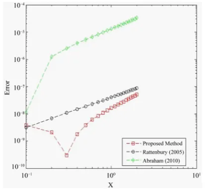
[image:8.595.210.419.514.705.2]Problem (72) is solved using the proposed ARK34 method. The results are obtained and compared with simi-lar ARK34 methods of [3] and [5] respectively and presented in Figure 1.
since it exhibits lesser error than the errors of the existing methods.
5. Conclusion
Two ARK methods are proposed, ARK3
(
s= =p 3)
and ARK34(
s=4,p=3)
. The methods have been proven to be consistent and stable, thereby guaranteeing their convergence. This is further illustrated by com-paring the performance of one of the methods with other methods of similar order. The proposed method ARK34 is shown to perform better than the existing methods.Acknowledgements
The authors would like to thank the reviewer(s) for their constructive criticisms.
References
[1] Lambert, J.D. (1991) Numerical Method for Ordinary Differential Systems: The Initial Value Problem. John Wiley & Sons Ltd., New York.
[2] Butcher, J.C. (1997) An Introduction to Almost Runge-Kutta Methods. Applied Numerical Mathematics, 24, 331-342.
http://dx.doi.org/10.1016/S0168-9274(97)00030-5
[3] Rattenbury, N. (2005) Almost Runge-Kutta Methods for Stiff and Non-Stiff Problems. Ph.D. Thesis, University of Auckland, Auckland.
[4] Abraham, O. and Adeboye, K.R. (2009) On the Derivation of Third-Order Almost Runge-Kutta (ARK) Methods with Four Stages (s = 4, p = 3). Proceedings of the 28th Annual Conference of Nigerian Mathematical Society, Ilorin, 23-27 June 2009, 42.
[5] Abraham, O. (2010) Development of Some New Classes of Explicit Almost Runge-Kutta Methods for Non-Stiff Dif-ferential Equations. Ph.D. Thesis, Federal University of Technology, Minna.
[6] Alimi, O.K. (2014) On the Performance of Richardson’s Extrapolation Technique in Estimating Local Truncation Er-rors for Explicit Almost Runge-Kutta Methods. Master’s Thesis, Federal University of Technology, Minna.
[7] Audu, K.J. (2015) Some Explicit Almost Runge-Kutta Methods for Solving Initial Value Problems. Master’s Thesis, Federal University of Technology, Minna.