Output Gap Estimation for Inflation
Forecasting: The Case of the Philippines
Bagsic, Cristeta and Paul, McNelis
Bangko Sentral ng Pilipinas
August 2007
Online at
https://mpra.ub.uni-muenchen.de/86789/
Bangko Sentral ng Pilipinas
BSP Working Paper Series
Center for Monetary and Financial Policy
Monetary Policy Sub-Sector
Out put Ga p Est im at ion for
I nflat ion Fore c a st ing:
T he Ca se of t he Philippine s
Paul D. McNelis and Cristeta B. Bagsic
August 2007
BSP Working Paper Series
Center for Monetary and Financial Policy
Monetary Policy Sub-Sector
Out put Ga p Est im at ion for
I nflat ion Fore c a st ing:
T he Ca se of t he Philippine s
Paul D. McNelis and Cristeta B. Bagsic
August 2007
Series No. 2007-01
The BSP Working Paper Series constitutes studies that are preliminary and subject to further revisions. They are being circulated in a limited number of copies for the purpose of soliciting comments and suggestions for further refinements.
The views and opinions expressed are those of the author(s) and do not necessarily reflect those of the Bangko Sentral ng Pilipinas.
ABSTRACT
This paper examines alternative estimation models for obtaining output gap measures for the Philippines. These measures are combined with the rates of growth of broad money, nominal wages and oil prices for forecasting inflation. We find that models which combine these leading indicators in a nonlinear way out-perform other linear combinations of these variables for out-of-sample forecasting performance.
TABLE OF CONTENTS
Abstract iii
List of Tables v
List of Figures v
1 Introduction 1
2 The Forecasting Process at the BSP 2
2.1 The Forecasting Models . . . 3
3 Use of Output Gap Among Central Banks 4 3.1 The Taylor Curve . . . 6
3.2 Central Bank Practices . . . 7
4 Output Gap Measures 9 4.1 HP Filter . . . 10
4.2 CES Production Function . . . 11
4.3 SVAR Approach . . . 12
4.4 Comparing Gap Estimates . . . 14
5 Inflation Forecasts 14 5.1 Alternative Models: Distilling Information from Indicators . . . 15
5.2 In-Sample Performance . . . 16
5.3 Out-of-Sample Performance . . . 17
6 Concluding Remarks 18 List of References 19 A Data 21 A.1 Constructed data . . . 21
A.2 Data Used in SVAR Estimation . . . 22
B Figures 23 LIST OFTABLES 1 Forecasting Performance Evaluation . . . 4
2 Survey of Use of Output Gaps Among Members of the Executives’ Meeting of East Asia-Pacific Central Banks (EMEAP) Group . . . 8
4 Point and Standard Errors of Impulse Responses . . . 14
5 Alternative Forecasting Models . . . 16
6 In-Sample Forecasts Evaluation . . . 17
7 Out-of-Sample Forecasts Evaluation . . . 17
LIST OFFIGURES 1 The Forecasting Process at the BSP . . . 23
2 Hodrick-Prescott Filter: Actual and Potential Output . . . 23
3 CES Production Function Estimates: Actual and Potential Output . . . 24
4 Structural Vector Autoregression (SVAR) Output Decomposition . . . 24
5 Output Gap Estimates Using HP Filter, CES Production Function, and SVAR . . 25
6 Linear Principal Components . . . 25
7 Nonlinear Principal Components . . . 26
8 Inflation and Inflation Forecasts: Upper and Lower Bounds . . . 26
Paul D. McNelis∗and Cristeta B. Bagsic†
August 2007
It is better to read the weather forecast before we pray for rain.
— Mark Twain
[M]easurement error has important effects for the appropriate conduct of the monetary authority as well as for policy performance. In most circumstances, an authority that takes explicit account of the uncertainty in the environment in which it operates is more successful than an authority that turns a blind eye to the issue.
– Orphanides, et al (2000)
1
Introduction
T
he output gap is an argument for the interest rate, along with current inflation and lagged interest rates, in most discussions of Taylor rules for central banks. The rationale is that a positive output gap is an indicator of inflationary pressure not seen in actual inflation. Yet, there is considerable uncertainty over the output gap and its key component, potential output. Does a rise or fall in current GDP mean a change in potential output or just a cyclical change in demand? These alternatives have different policy implications. Central banks can raise interest rates to curb a rise in demand but cannot affect potential output.In this paper we examine three measures for obtaining potential output – and thus the output gap – for the Philippine economy. These measures are the Hodrick-Prescott (HP) filter, the constant elasticity of substitution (CES) production function, and the structural vector
∗Department of Finance, Fordham University, New York. [email protected]. McNelis’ work was supported
by the United States Agency for International Development under the EMERGE Project in Manila during 2005-2006.
†Center for Monetary and Financial Policy, BSP. [email protected]. The authors thank Haydee Ramon for
autoregressive (SVAR) approaches for obtaining measures of the output gap. We find that all three measures help forecast inflation. We argue that the BSP should adopt a “thick model” approach to output gap estimation for inflation forecasting, making use of all of these measures as well as information from the rates of growth of broad money, nominal wages, and the price of oil.
To put the main purpose of our paper in perspective, we first take a look at the role of the inflation forecasting process within the policy-setting framework at the Bangko Sentral ng Pilipinas. In Section 3 is a brief survey of theoretical and empirical issues concerning the role of output gap estimates in the inflation targeting (IT) regime, and the results of an informal survey we conducted among selected central banks that estimate the output gap. Section 4 presents our alternative measures of the output gap. We turn to models of inflation, both for in-sample understanding and for out-of-sample forecasting in Section 5. Section 6 concludes.
2
The Forecasting Process at the BSP
The inflation targeting (IT) framework is implemented in the Philippines by announcing the inflation target two years ahead. For instance, the annual target of 4 percent for 2008 was announced in December 2006.1 As a consequence, policy discussions in the BSP are gen-erally focused on monthly forecasts two years forward of the inflation rate, as well as on the developments and outlook for economic variables that help predict inflation on the one hand, and decision variables on the other.
Throughout the policy-setting process, the synergy between seasoned judgment of both the modelers and decision makers, and the quantitative tools is apparent. The models, in particular, both shape and are refined by consultations and discussions at various levels. To arrive at the inflation targets and the inflation forecasts, the BSP typically follows the process shown in Figure 1.2
The forecasting process follows the decision making cycle for monetary policy. Policy meet-ings are held at an interval of six weeks. Before each meeting, the Technical Staff prepares a policy decision support paper for submission to the Advisory Committee, an internal body composed of senior officials tasked to submit recommendations on monetary policy to the Monetary Board. The Advisory Committee discusses the contents of the policy paper, which reviews recent developments concerning conditions pertaining to, among other things, aggre-gate demand, supply-side conditions, the labor market, domestic liquidity, financial markets,
1Starting December 2006, the inflation target announced is the midpoint of a two-percentage-point spread.
Pre-viously, targets were in the form of a one-percentage-point-thick range. See BSP Media Release of 14 December 2006 for details on the shift.
2The BSP is instrument independent but is goal dependent. Thus, in setting the inflation targets, the illustrated
and the global economy. The Committee also discusses the outlook for inflation, starting with the latest forecasts prepared by Bank staff along with the emerging risks to future inflation and other information relevant to the policy stance. On the basis of its view of the inflation outlook and prevailing economic conditions, the Advisory Committee formulates a policy recommen-dation to the Monetary Board. If necessary, the forecasts are revised to reflect important new information that becomes available prior to the policy meeting of the Monetary Board later in the same week.
At the policy meeting of the Monetary Board, the Deputy Governor for monetary policy presents to Monetary Board the information contained in the policy paper, which incorporates the comments as well as the recommendations of the Advisory Committee. The Monetary Board then makes its decision on the stance of monetary policy on the basis of the inflation forecasts and its assessment of the balance of risks to inflation as well as other information made available during the discussion.
2.1 The Forecasting Models
The BSP currently uses two forecasting models: its Multi-Equation Model (MEM) and its Single Equation Model (SEM). The MEM has eight (8) behavioral equations and four (4) identities. Meanwhile, the SEM has inflation rate in its left-hand side; and financial depth measured by M4/nominal GDP, the national government’s cash position, 91-day Treasury bill rate, domestic oil price, nominal wage, non-oil import prices and a dummy for the rice crisis in 1995 as explanatory variables. Both of these models give monthly forecasts of the CPI inflation rate.
Aside from being the richer model, the MEM captures output gap, albeit in a limited way. The deviation of agricultural production from trend is one of the explanatory variables in the inflation equation in the MEM.3
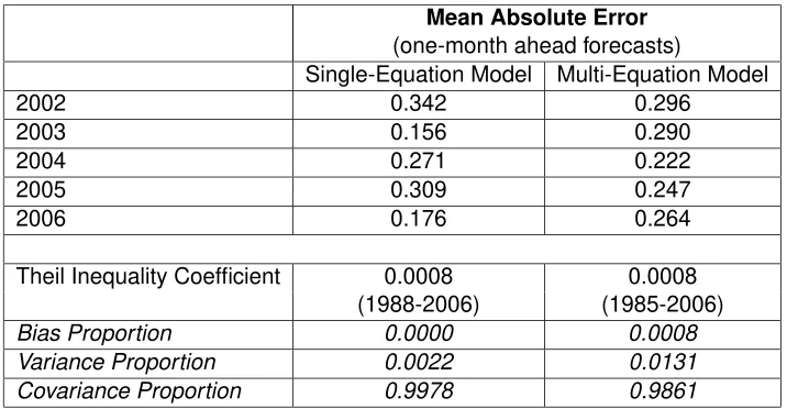
Table 1 shows the forecasting performance of the models of the BSP in the last five (5) years. The mean absolute error (MAE) is the 12-month average of the monthly absolute errors for one-month ahead forecasts. The absolute error is computed as the difference in percentage points between the absolute value of actual inflation and the forecast of inflation for month t
conditional on information available in montht−1.
In effect, over the last five (5) years, the BSP’s monthly one-period ahead forecasts are on average 0.156 - 0.342 percentage points away from actual inflation. The covariance propor-tions cited in Table 1 indicate that the remaining forecasting errors of both models are more than 98 percent unsystematic. More importantly, the Theil inequality coefficient is very close to zero.
The MEM’s structure and forecasting performance, meanwhile, has made it the default workhorse for policy simulations at the BSP. BSP analysts have primarily used the MEM for quantitative predictions of the lagged effects of policy actions on inflationary developments
3Refer to BSP’s First Quarter 2007 Inflation Report, which is available in its website www.bsp.gov.ph, for the
Mean Absolute Error
(one-month ahead forecasts)
Single-Equation Model Multi-Equation Model
2002 0.342 0.296
2003 0.156 0.290
2004 0.271 0.222
2005 0.309 0.247
2006 0.176 0.264
Theil Inequality Coefficient 0.0008 0.0008
(1988-2006) (1985-2006)
Bias Proportion 0.0000 0.0008
Variance Proportion 0.0022 0.0131
Covariance Proportion 0.9978 0.9861
[image:10.612.144.502.122.308.2]Source: Department of Economic Research-Bangko Sentral ng Pilipinas
Table 1: Forecasting Performance Evaluation
and, in turn, on the real economy and BSP’s decision variables. Nevertheless, and in recog-nition of these various and variable lags and of current advances in research and computing technologies, research and modeling resources have lately been employed to enhance the forecasting power of BSP’s other model – the annual Long Term Macro Model (LTMM) – and to develop new ones that can better explain the transmission channels of policy actions to the real economy.
The BSP’s research agenda and institutional plans reflect a strategy for enhancing model-ing capacity over the next five (5) years. The accuracy and performance of the current crop of models are assessed on an on-going basis. More importantly, models are updated or devel-oped at the instance of either the Board, senior management, or the technical staff. Starting in late 2005, forecasting, and model updating and development have been assigned to two different units in order to give equal emphasis to both activities. The extensive job of making periodic forecasts of economic and financial variables has been given to the newly-created Economic and Financial Forecasting Group (EFFG). On the other hand, the tasks of updating current models and developing new ones (like the current subject model for output gap estima-tion) have been assigned to the, also newly-created, Center for Monetary and Financial Policy (Center from hereon).
3
Use of Output Gap Among Central Banks
demand to inflation; and the exchange rate channel to aggregate demand to inflation.
The transmission channels to AD are also the channels to the output gap. Higher AD will increase the output gap, which can then lead to an increase in inflation as higher production increases the costs of production, and higher demand allows firms to increase prices. In the long term, monetary policy can, at best, provide a stable environment for the real economy Bad and volatile monetary policy generates a macroeconomic environment that discourages investment and, therefore, growth in potential output.
As Taylor (2000) has pointed out, the “output gap is a key variable in most policy rules, but it is important whether or not a central bank follows a policy rule”. (p.17) The value of an output gap measure to a central bank is in the signal it may provide about developments in future inflation.
Output gap is typically defined as the percent difference between actual output and poten-tial output. Potenpoten-tial output is the output that the economy can produce at full employment. It is also seen as the level of output that is compatible with a stable rate of inflation. A positive output gap indicates inflation pressure not seen in actual inflation. However, because potential output is unobserved, different estimation models can give divergent estimates of output gaps for a given economy.
It cannot be overemphasized that output gap estimation is not without a lot of uncertainties. According to Orphanides, et al (2003), the “most problematic element associated with real-time estimates of the output gap is that it is based on end-of-sample estimates of an output trend (potential output), which are unavoidably highly imprecise”. Current period estimates of the output gaps generally are based on forecasts of current period actual and potential GDP. Once the data on GDP (and the other variables used to estimate potential output) become available in the following quarter, they may still be preliminary for sometime and quite likely to be revised. At the same time, updating the model for one more data point once the statistics for the following period become available could also affect the trend. Another possible source of measurement error is the model used, as when the central bank uses a model it believes give the true gap when in fact it does not.
The accuracy of output gap estimates acquires added importance to a monetary authority which explicitly includes output gap in its loss function. Even so, Taylor (2000) finds that despite the difficulty associated with output gap estimation, monetary authorities must respond to it. “Pre-emptive strikes – such as that taken in the United States in the late 1980s and not taken (at least [not] soon enough or large enough) in Japan in the late 1980s – require that the central bank begin to raise interest rates when the output gap increased [...] even though there may not be a noticeable movement in inflation.” (p.17)
measurement error in the output gap becomes large, the efficient Taylor rule parameter on the output gap could fall to zero.” He clarified, however, that “uncertainty in the output gap does not affect optimal central bank behaviour in a linear-quadratic framework [even as] it can have significant effects on restricted instrument rules such as the Taylor rule.” (p.15)
While it is true that accurate estimates of current period output gap is of immense interest to policymakers, forecasts of future-period output gaps also provide additional insights. Simu-lating expected paths of output gap given various policy action options would help clarify the decision-making process. Therefore, resolving the typical end-sample problem, exhibited by univariate filters for instance, though necessary, will not be sufficient to address fully the policy dilemma.
3.1 The Taylor Curve
The Taylor curve describes a negative relationship between inflation rate volatility and output growth volatility where output volatility is in the y-axis and inflation rate volatility is in the x-axis.4
Strict inflation targeting implies an aggressive and volatile policy stance leading to considerable volatility in interest rates and the exchange rate that will then result to higher volatility of output. Flexible inflation targeting has price stability in the form of an inflation target as its primary goal; but gives some consideration to stabilizing output movements around potential output. This means allowing a longer time horizon to achieving the inflation target than what is technically doable.
Should an inflation targeting central bank also attempt to stabilize output? More categorical still, does output stabilization enhance an IT framework? Debelle (1999) succinctly illustrated the role of output stabilization in an inflation-targeting policy environment. He illustrated the objective function of an IT central bank using the following simple model which consists of the Phillips curve, an aggregate demand function, and the central bank’s loss function, respec-tively, as follows:
πt =πt−1+α
yt−1−yt∗−1
+εt (1)
yt=y∗t +β
yt−1−yt∗−1
−γ(rt−1−r∗) +ηt (2)
Lt=Et
∞
s=t
δs−t(1−λ) (πs−π∗)2+λ(ys−ys∗)
2
(3)
Adopting Debelle’s (1999) notations,πis inflation,π∗ is the inflation target,yis output,y∗
is potential output,r is the short-term real policy rate,δ is a discount rate, andεt andηt are
independent and identically distributed shocks, andr∗is the neutral real interest rate.
Note that two-period ago short-term real interest rate affects one-period ago output, which in turn affects current period inflation rate. Economists have pointed to this difference in lag structure as the basis of the tradeoff.
The above model solves r, thus:
rt=r∗+ϕ1(πt−π∗) +ϕ2(yt−yt∗) (4)
The output gap is thus incorporated in a Taylor-type reaction function (Equation 4), which could be used in either a positive or a normative manner.
Previous studies have concluded that IT is enhanced by keeping in check output volatil-ity. Assuming that monetary policy affects the real economy in the short run, strict inflation targeting leads to changes in interest rates and, in effect, the foreign exchange as often as the number of times that inflation deviates from target.5 Strict inflation targeting requires that
deviations of actual inflation from target be eliminated at a minimum period and without regard to impact on growth. This implies volatile interest rates, foreign exchange, and output. The in-duced volatility in interest rates and foreign exchange could eventually translate to instrument instability. On the other hand, wild fluctuations in output performance are inimical to welfare maximization. In any case, even when a central bank chooses to be a strict inflation targeter – formally, it is when the deviation of actual output from potential has zero weight in its objective function – the output gap still has information content because it portends inflation expecta-tions. However, to be relevant to monetary policy decision makers, estimates must go beyond that of the historical series. For example, the estimates of the current gap and expected output gap given alternative policy actions would be useful.
In the same vein Svensson (2002) found that flexible IT provides the greatest benefit com-pared to strict inflation targeting and strict output targeting. A target horizon of one to two years is one of the imprints of a flexible IT regime.6
Nonetheless, Debelle (1999) cites that even for strict inflation targeters (where the central bank’s loss function gives zero weight to deviation of output from potential), output gap is useful. Output gap signals inflation expectations. Put simply, a positive output gap portends inflationary pressure (i.e., either rising inflation rate or accelerating inflation rate).
3.2 Central Bank Practices
Using Philippine data, Yap (2003) concludes that the output gap has a role to play in the Philip-pine IT framework. He observes that including the output gap variable in an inflation model (a two-step error correction model, with Dubai crude oil, exchange rate and money supply on the right hand side) for the Philippines improves its performance, e.g., higher adjustedR2. He uses three measures of output gap: a time trend model, an unobserved component method, and the H-P filter.
5For instance, see Svensson (2002).
Estimation Methodology Estimation Frequency Publication Frequency Reserve Bank of Australia Production Function Quarterly (since mid 90s) Not regularly.
Multi-variate HP filter
People’s Bank of China Production Function Quarterly (2001) Internal use. State-space estimation
Hong Kong Monetary Authority Production Function Quarterly (2001) Internal use. Bank Indonesia SVAR Quarterly (1999) Internal use. Bank of Japan Production Function Quarterly (2003) 2x/year Bank Negara Malaysia Production Function Quarterly (1998) annual
Multi-variate HP filter
Reserve Bank of New Zealand Multi-variate Quarterly Not regularly. HP filter
Monetary Authority of Singapore Multi-variate HP filter Quarterly Not regularly. HP filter
[image:14.612.110.544.122.319.2]Variable Span Smoother
Table 2: Survey of Use of Output Gaps Among Members of the Executives’ Meeting of East Asia-Pacific Central Banks (EMEAP) Group
Inflation targeting central banks that use output gaps include, among others: the Bank of England, Bank of Canada (BoC), Reserve Bank of New Zealand (RBNZ), Reserve Bank of Australia (RBA), Bank Indonesia, Bank of Norway, and the Sveriges Riksbank.
The Reserve Bank of New Zealand estimates output gap using a multivariate filter, which, in the case of New Zealand, is a Hodrick-Prescott (H-P) filter augmented with residuals from a Phillips curve relationship and two Okun’s law equations (unemployment gap and capacity utilization gap). The output gap has been a considerable factor in RBNZ’s structural macro-model. (Graff, 2004)
The Bank of Canada, meanwhile, has used a structural vector autoregression approach and extended multivariate filter to estimate output gap. (Rennison, 2003) It incorporates an output gap variable in the reaction function embedded in its Quarterly Path Model. (Longworth and Freedman, 2000)
On the other hand, the Riksbank publishes three output gap measures in its Inflation Re-port: the H-P filter (with smoothing parameter of 6400), an unobserved component measure using an Okun’s Law and Phillips curve relationships to extract the cyclical component of out-put from inflation and unemployment, and a production function model which uses capital stock and employment data to estimate potential output. The output gap is used to assess inflationary expectations. (Sveriges Riksbank, 2005)
Table 2 shows the results of an informal survey conducted by the BSP on members of the Executives’ Meeting of East Asia-Pacific Central Banks (EMEAP) group. Among the re-spondents, the production function approach to estimating output gap is the most prevalent, followed by the use of the multivariate Hodrick-Prescott filter. Quarterly estimation is favored. Lastly, none of the eight (8) respondents have made output gap an official statistic.
4
Output Gap Measures
Prevalent theory assumes that output gap accounts for a portion of the transitory or cyclical portion of real output. Viewed another way, output gap is that component of actual output arising from demand shocks. The output gap is, likewise, deemed as the portion of real output that is associated with unanticipated inflation.
According to Orphanides, et al (1999), the “difficulties [in measuring potential output] spring from a certain fundamental ambiguity in the concept of potential aggregate output. [. . . ] the economy’s productive potential is typically defined as the trend component of actual output, with trend estimated in various ways. Alternatively, potential output is inferred from the behavior of inflation”. (p.4)
In general, the data determine the appropriate output gap measure. Broadly speaking, the methodologies used in the estimation of potential output may be classified into two: statisti-cal detrending techniques, and methodologies that link potential output with other economic variables as dictated by economic theory. Statistical detrending techniques decompose a time series into permanent and cyclical components. Examples of these techniques are: Hodrick-Prescott (H-P) filter, Beveridge-Nelson decomposition, and various unobserved components methods. On the other hand, the structural VAR, production function, and multivariate system models use economic theory to separate the impacts of structural and cyclical components of output. Examples of output gap measures which decompose the output into its trend and cycle components are:7
1. linear trend method: ordinary least squares (OLS), with linear deterministic trend
2. quadratic trend method: OLS, with quadratic deterministic trend
3. breaking linear trend model: OLS, incorporates structural breaks/slowdowns
4. Hodrick-Prescott model: based on the filter proposed by Hodrick and Prescott in 1997 with their recommended smoothing parameter of 1600 for quarterly data
5. band-pass filter method
6. Beveridge-Nelson method: models output as an ARIMA(p,1,Q) series
7. unobserved components model:
(a) univariate models:
i. Watson method: models the output trend as a random walk with drift and the cyclical component as a stationary AR(2) process
ii. Harvey-Clark model: follows the Watson method but does away with the as-sumption of a constant drift in the trend component
iii. Harvey-Jaeger method: has the same trend component as the Harvey-Clark model but assumes a cyclical component that is a stochastic process
(b) multivariate models
i. Kuttner model: adds a Phillips curve to the Watson method
ii. Gerlach-Smets method: adds a Phillips curve to the Harvey-Clark model
8. Blanchard and Quah’s structural vector autoregression (SVAR) model: imposes long-run restriction on output to a VAR system. One obvious advantage of SVAR measure, in general, is that they do not suffer end-of-sample problems. They are also able to forecast expected output gaps.
9. Cochrane method: a two-variable VAR that estimates the permanent and cyclical com-ponents of output. This approach exploits the permanent-income hypothesis, and is founded on the assumptions that (i) consumption and GNP are cointegrated, and (ii) consumption follows a random walk process.
10. Production function approach: generally implemented by calculating potential output given the trends in employment and capital.
For this exercise we used the HP filter, CES production function, and SVAR to estimate the output gap for the Philippines. We discuss our three alternative measures and show quantita-tive estimates for the output gap below.
4.1 HP Filter
This method is between and betwixt detrending and first differencing of data. The advantage is that it is easy and quick to use. The following equation describes the filter:
M in
x
t=0
(yt−yxt) +ω x
t=0
ytx+1−yxt
−ytx−yxt−1
2
(5)
The parameterωis the controlling parameter for the smoothness of the trend. It is usually set at 1600. The output gap is defined simply asyt−yxt, the difference between actual log
output less the smoothed trend output. This is clearly a mechanical device which defines cycles it extracts by the choice of the smoothing parameterω.
shock. In other words, it is penalized for changing the trend. However, at the end of the sample, this disincentive is absent.
Actual and potential output appear in Figure 2.
4.2 CES Production Function
The Constant Elasticity of Substitution production function was originally developed by Arrow, Chenery, Minhas and Solow (1961) as an alternative to the more familiar Cobb-Douglas pro-duction function. It has the following functional form:
Yt=AZt
(1−α)L−tκ+αKt−κ−1κ (6)
The variableZt is the aggregate total factor productivity shock,Ais a constant term, while
α,(1−α)represent the coefficients for capitalKand laborL, known as distribution parameters which explain the relative factor shares in total output. The parameter κ is the substitution parameter.
The CES production yields the following equations for the marginal products of labor and capital:
∂Yt
∂Lt
=A1−κZ1−κ t (1−α)
Y t Lt κ+1 (7) ∂Yt ∂Kt
=A1−κZt1−κα
Y
t
Kt
κ+1
(8)
The elasticity of substitution of capital and labor, symbolized byηK,L, is given by:
ηK,L=
1
1 +κ (9)
A necessary condition for a unique steady-state is thatκ≤0. This CES function reduces to the Cobb-Douglas log-linear function under the assumption thatκ= 0.
Using a second-order Taylor expansion of equation (6) with the dependent variable re-defined as yt = Yt/Lt, with kt = Kt/Lt, and assuming Constant Returns to Scale, the CES
function takes the following form:
log(yt) = log(A) +λ·tr+αlog(kt)−.5κα(1−α) [log(kt)]2+ǫt (10)
The parameterλpicks up a trend term.
series. On the other hand, the production function model suffers from the fact that the series needed to estimate it, especially in emerging economies, are generally of poor quality or even unavailable.
We define the output gap as the residual betweenlog(yt)andlog(yt), or simplyǫt. This is
not the normal practice. If measures of capacity utilization and full-employment were available, we could use the estimated production function to generate potential output under assumptions of full capacity utilization and non-accelerating inflation full employment. In this case, actual utilized labor and estimates of the capital stock are available; however, structural unemploy-ment rate is not available. The capital utilization rate is available only for the manufacturing sector starting late 1990s.
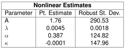
Table 3 gives the estimates for the CES production function coefficients for equation (10). Only the time trend,λ, is statistically significant. Nonetheless, the parameterκis close to zero and negative, implying a unique steady-state and an elasticity of substitution between capital and labor of greater than unity.
Actual and potential output estimates are plotted in Figure 3.
Nonlinear Estimates
Parameter Pt. Estimate Robust St. Dev.
A 1.76 290.53
λ 0.0045 0.0018
α 0.387 124.82
[image:18.612.216.429.357.439.2]κ -0.0001 147.96
Table 3: CES Production Function
4.3 SVAR Approach
The structural vector autoregression (SVAR) method uses a wider set of variables, not just output, capital, labor, and trend terms. It is based on a vector autoregressive model of the form:
[I−A(L)]Yt=ut (11)
whereA(L)is a lag operator,Y a matrix of endogenous variables, andua matrix of residuals. Equation (11) is known as the Reduced Form (RF)Model. The idea behind this approach is to convert the multivariateARgiven by equation (11) into a restricted Wold moving average
(M A)process:
Yt = [I−A(L)]−1ut
We impose linear restrictions relating the innovations of the MA processεtto the residuals
of the reduced form estimated VAR model at timet,ut, for ak−variable model:
εt = S(0)ut
E(εt, ε′t) = S(0)E(utu′t)S′(0) = Σ.
The basic point of SVAR estimation is simple and straightforward. Knowledge ofS(0), the matrix of contemporaneous effects of the structural disturbancesεt onYt allows us to recover
the structural shocks from the reduced-form residuals ut. In estimating the SVAR, we first
estimate a Bayesian VAR model. The logarithm of output enters in first-differences and is the first variable in the model.
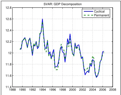
Thus, changes in potential output∆gdppand the output gap∆gdpg can be written as:
∆gdpp=S
11(0)ε1,t+S11∗ (L)ε1,t (12)
∆gdpg=S12(L)ε2,t+. . .+S1k(L)εk,t (13)
The model tells us that the permanent component of changes in actual GDP is simply its own current and lagged innovations or shocks. This represents the non-cyclical, permanent innovations to real GDP coming from purely exogenous technological change or other sources beyond the control of policy. The cyclical component of the change in GDP is explained by the lagged (not current) values of other variables in the model.
It is important to note that potential GDP and the GDP gap are presented as first differ-ences, not in terms of levels. We can convert these into levels by starting from an initial estimate oflog(gdp). The calculation of the output gap is within the structure of the VAR/SVAR model. We do not compare actual output with a trend level or level of output from a production function. We simply compare the output generated by permanent shocks to GDP with the level of output generated by cyclical or demand-side variables within the VAR framework. It is conceptually different from the HP and CES measures.
In the SVAR estimation, we use the following seasonally adjusted variables: the logarithmic change in real GDP,∆y, the logarithms of the real exchange rate and employment, given by RER, and L; the rate of interest, WAIR; and the deficit/GDP ratio, given byDEF GDP.
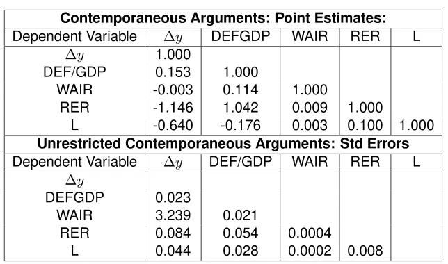
Table 4 gives the point estimates for the SVAR estimation. We see that DEF GDP is positively affected by innovations in∆y. Meanwhile,W AIRhas a negative relationship to the contemporaneous shocks toδy, and positive relationship withDEF GDP. According to our model, a positive shock to∆ywill tend to depreciate theRERduring the same period, while
RERhas a positive relationship with innovations to DEF GDP andW AIR. Positive shocks to∆yandDEF GDP have a negative effect onLduring the same period. On the other hand,
Lis positively related to shocks toW AIRandRER. Table 4 gives the standard errors of the point estimates.
Contemporaneous Arguments: Point Estimates:
Dependent Variable ∆y DEFGDP WAIR RER L
∆y 1.000
DEF/GDP 0.153 1.000
WAIR -0.003 0.114 1.000
RER -1.146 1.042 0.009 1.000
L -0.640 -0.176 0.003 0.100 1.000
Unrestricted Contemporaneous Arguments: Std Errors
Dependent Variable ∆y DEF/GDP WAIR RER L
∆y
DEFGDP 0.023
WAIR 3.239 0.021
RER 0.084 0.054 0.0004
[image:20.612.162.484.117.307.2]L 0.044 0.028 0.0002 0.008
Table 4: Point and Standard Errors of Impulse Responses
4.4 Comparing Gap Estimates
Figure 5 presents all three gap measures. These are the gap measures for the full sample. We see that the SVAR measure is considerably more volatile than the HP and CES measures.
The dip in the early 1990s seen in the output gaps estimated using Equations (5) and (6) reflects the power crisis that saw widespread power outages in the Philippines during the pe-riod. Its resolution and the subsequent market reforms coincided with the rise in the output gaps from these measures. The period of the Asian crisis and the subsequent El Ni˜no episode show declining HP and CES output gaps once again. In contrast, the SVAR output gap de-clined much earlier and spiked as the other two measures bottomed. Interestingly, the SVAR results during this period are consistent with the rising inflation rate.
More recently, even as all three measures show positive gaps for estimation done until Q3 2006, they are also all starting to turn southwards.
5
Inflation Forecasts
The proof of the pudding is in the eating: how well do these alternative measures help forecast inflationary developments? We do not know what exactly the “output gap” is, so why not use all three? We find that all three are helpful for recursive out of sample forecasts. For in-sample forecasts, the HP and CES are significant but the SVAR measure is not. But the best overall model for forecasting is one which uses information from all three measures as explanatory variables.
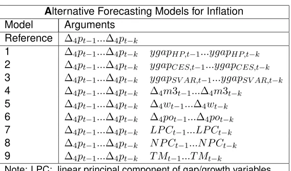
of inflation. We then explore alternative models: (1) lags of inflation and HP gap; (2) lags of inflation and CES gap; (3) lags of inflation and SVAR gap.
We also make use of additional leading indicators: the annualized rates of growth of broad money ∆4m3t = (m3t −m3t−4), nominal wages ∆4wt = (wt −wt−4), and the price of oil
∆4pot= (pot−pot−4).
Additionally, we used linear and non-linear principal components to “distill” one measure from all three, and used these alternatives. In all of our model, we define inflation as as
pt−pt−4.
5.1 Alternative Models: Distilling Information from Indicators
Stock and Watson (2000) have shown that the best way to forecast inflation is to combine information from a wide class of potential leading indicators or explanatory variables. We have six possible indicators: the three output gap measures, as well as the rates of growth of broad money, wages and the price of oil.
One way to combine the information from these variables is to make use of principal com-ponent methods.
Linear principal components for a set of variables is equivalent to a series of orthogonal regressions. Given a data set X consisting of T observations for H variables, we find the first principal component by computing the eigenvalues and eigenvectors from the following equation:
[X′X−νiI]Vi= 0
whereνi is the i-th eigenvalue andVi is the associated eigenvector of dimension (H by 1) for
eigenvalueνi. For linear principal components, the first linear principal component is simply
the matrixX multiplied by the eigenvector associated with the first or largest eigenvalue,V1:
P C1=X·V1
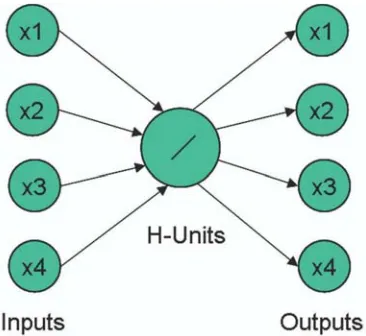
For a matrix of rankH, there can be at mostHeigenvalues. Figure 6 illustrates the setup of linear principal components. The variablesx1throughx4map into each other through the H-unit set of principal components.
An alternative to linear principal components is the use of nonlinear auto-associative maps. Just as in linear principal components, the variablesx1throughx4map into each other. Figure 7 shows one example of a nonlinear principal component. The variablesx1, ...x4map into each other, as before, but they do so through a set of encoding receptors, usually logistic functions, represented by the boxesc11andc12, onto at mostH−units, whereH = 4. TheH−units
Alternative Forecasting Models for Inflation
Model Arguments
Reference ∆4pt−1...∆4pt−k
1 ∆4pt−1...∆4pt−k ygapHP,t−1...ygapHP,t−k
2 ∆4pt−1...∆4pt−k ygapCES,t−1...ygapCES,t−k
3 ∆4pt−1...∆4pt−k ygapSV AR,t−1...ygapSV AR,t−k
4 ∆4pt−1...∆4pt−k ∆4m3t−1...∆4m3t−k
5 ∆4pt−1...∆4pt−k ∆4wt−1...∆4wt−k
6 ∆4pt−1...∆4pt−k ∆4pot−1...∆4pot−k
7 ∆4pt−1...∆4pt−k LP Ct−1...LP Ct−k
8 ∆4pt−1...∆4pt−k N P Ct−1...N P Ct−k
9 ∆4pt−1...∆4pt−k T Mt−1...T Mt−k
[image:22.612.182.466.119.286.2]Note: LPC: linear principal component of gap/growth variables NLP: non-linear principal component of gap/growth variables TM: trimmed mean of gap, growth, LPC, NPC variables
Table 5: Alternative Forecasting Models
We combine the three output gaps and the three growth rates for a nonlinear principal component to see if this provides additional information not gleaned by the linear principal component.
Finally, using all the information from the three output gaps, the three growth rates, the linear and nonlinear principal components, we construct a trimmed mean (the mean cutting out the highest and lowest 10% outliers), to form a single leading indicator that we use in Model 9.
We summarize the models we use in Table 5.
5.2 In-Sample Performance
Before evaluating the forecasting performance, we first examine the performance of the model on the full data set. The results appear in Table 6. We should note that the data we use in the in-sample estimation differ from the data used in forecasting. In forecasting arguments, the output gaps are recursively updated. We do not use the full-sample output gaps as arguments for forecasting inflation in earlier periods of the model.
Reference 1 2 3 4 5 6 7 8 9 RSQ 0.921 0.927 0.924 0.925 0.930 0.937 0.933 0.924 0.925 0.928
Granger Tests of Causality Model
1 2 3 4 5 6 7 8 9
[image:23.612.120.522.124.206.2]p-values 0.593 0.898 0.806 0.386 0.070 0.190 0.882 0.836 0.512
Table 6: In-Sample Forecasts Evaluation
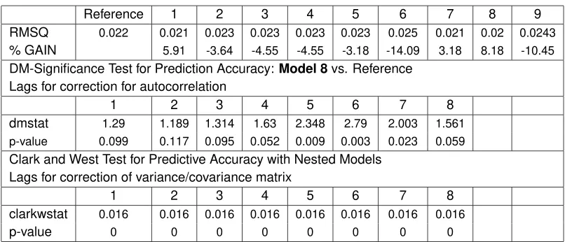
Reference 1 2 3 4 5 6 7 8 9
RMSQ 0.022 0.021 0.023 0.023 0.023 0.023 0.025 0.021 0.02 0.0243
% GAIN 5.91 -3.64 -4.55 -4.55 -3.18 -14.09 3.18 8.18 -10.45
DM-Significance Test for Prediction Accuracy:Model 8vs. Reference Lags for correction for autocorrelation
1 2 3 4 5 6 7 8
dmstat 1.29 1.189 1.314 1.63 2.348 2.79 2.003 1.561 p-value 0.099 0.117 0.095 0.052 0.009 0.003 0.023 0.059
Clark and West Test for Predictive Accuracy with Nested Models Lags for correction of variance/covariance matrix
1 2 3 4 5 6 7 8
clarkwstat 0.016 0.016 0.016 0.016 0.016 0.016 0.016 0.016
p-value 0 0 0 0 0 0 0 0
Table 7: Out-of-Sample Forecasts Evaluation
5.3 Out-of-Sample Performance
[image:23.612.121.524.253.426.2]6
Concluding Remarks
The uncertainties in output gap estimation arise from model selection and data issues. For example, statistical issues such as data quality and data revisions have been known to contra-dict prior appreciation of output gap estimates. It is in this context that the Philippine monetary authorities will find the use of a “thick model” attractive, if not a necessity during periods when indicators of inflation do not all point in one direction.
This study does not make any determination on how much weight the central bank should accord the output gap in setting the policy stance. The determination of such weight, as well as exercises to measure the degree of uncertainty arising from data revision and model selection, and to remedy data weaknesses, is a subject for future research.8
Given the significant relationship between Philippine inflation rate and the output gap, ef-forts to better understand and improve estimates of the output gap should serve the BSP well. We conclude, in the spirit of Sargent, Williams and Zha (2004) that it is important to acknowledge model uncertainty about the formation of output gap measures in the formulation of monetary policy, and make use of thick models, or combinations of models.
8In a comment to the authors, BSP Monetary Board Member Vicente B. Valdepe
LIST OFREFERENCES
[1] Arrow, K.J., H.B. Chenery, B.S. Minhas, and R.M. Solow (1961), “Capital-Labor Substitu-tion and Economic Efficiency”, Review of Economics and Statistics 43, 225-250.
[2] Clark, T.E. and K. D. West (2004), “Using Out-of-Sample Mean Squared-Prediction-Errors to Test the Martingale Difference Hypothesis”. Working Paper, Department of Economics, University of Wisconsin.
[3] Claus, I. (2003), “Estimating Potential Output for New Zealand”, Applied Economics, 35, 751-760.
[4] Debelle G. (1999), “Inflation Targeting and Output Stabilization”, Reserve Bank of Aus-tralia Research Discussion Paper, 1999-08.
[5] Diebold, F X. and R. Mariano (1995), “Comparing Predictive Accuracy”, Journal of Busi-ness and Economic Statistics, 3, 253-263.
[6] Duffy J., and C. Papageorgiou (2000), “A Cross-Country Empirical Investigation of the Aggregate Production Function Specification”, Journal of Economic Growth, 5, 87-120.
[7] Graff, M. (2004), “Estimates of the output gap in real time: how well have we been doing?”, RBNZ Discussion Paper Series, 2004/04.
[8] Joseph, C., J. Dewandaru and I. Gunadi (2003), “Playing Hard or Soft? : A Simula-tion of Indonesian Monetary Policy in Targeting Low InflaSimula-tion Using A Dynamic General Equilibrium Model”, Paper presented in EcoMod2003 International Conference on Policy Modeling held in Istanbul on 3-5 July 2003.
[9] Longworth, D. and C. Freedman (2000), “Models, Projections, and the Conduct of Policy at the Bank of Canada”, Paper prepared for the conference “Stabilization and Monetary Policy: The International Experience”, organized by Banco de Mxico to celebrate its 75th anniversary, 14-15 November, 2000.
[10] Orphanides A. (2003), “Historical Monetary Policy Analysis and the Taylor Rule”, Journal of Monetary Economics 50, 983-1002.
[11] , R. Porter, D. Reifshneider, R. Tetlow, and F. Finan (2000), “Errors in the Measure-ment of the Output Gap and the Design of Monetary Policy”, Journal of Economics and Business, 52, 117-141.
[12] , S. van Norden (2005), “The Reliability of Inflation Forecasts Based on Output Gap Estimates in Real Time”, Journal of Money, Credit and Banking, Ohio State University Press, vol. 37(3), pages 583-601, June.
[13] Rennison, A. (2003), “Comparing Alternative Output-Gap Estimators: A Monte Carlo Ap-proach”, Bank of Canada Working Paper 2003-8.
[15] Smets, F. (1998), “Output Gap Uncertainty: Does It Matter for the Taylor Rule?”, BIS Working Paper 60.
[16] Stock J.H, and M.W. Watson (2000), “Forecasting Inflation”, Journal of Monetary Eco-nomics, 44, 293-335.
[17] Svensson, L.E.O. (2002), “Monetary Policy and Real Stabilization”, paper presented at the conference “Rethinking Stabilization Policy”’, A Symposium Sponsored by the Federal Reserve Bank of Kansas at Jackson Hole, Wyoming on August 29-31, 2002.
[18] Sveriges Riksbank (2005), “Inflation Report”
[19] Taylor, J B. (1979), “Estimation and Control of a Macroeconomic Model with Rational Expectations”, Econometrica, 47, 1267-1286.
[20] (1993), “Discretion vs. Policy Rules in Practice”, Carnegie-Rochester Conference Series on Public Policy 39, 195-214.
Appendix
A
Data
A.1 Constructed data
Labor
To estimate the full-time equivalent employment level, L, quarterly data on mean hours worked per sector, and the number of employed who reported for work per sector are used. It is assumed that one who is employed full-time works for 40 hours per week.
Procedure in CalculatingLt
1. Get the sum of the number of employed who reported for work for sectori,EWi,t.
EWi,t=
EWi,thrs (14)
whereEWhrs
i,t denotes the number of employees in sectoriwho worked for one of the
followinghrscategories:<20 hours, 20-29 hours, 30-39 hours, and≥40 hours.
2. Calculate the weight for each sector,wi,t, by dividing the actual mean hours of sectori,
meani,tby 40 hours.
wi,t=
meani,t
40 (15)
3. Calculate the full-time equivalent employment level for each sector.
Li,t=EWi,t×wi,t (16)
4. Ltis the sum ofLi,tacross alli’s.
Capital
In calculating the capital stock for the quarter, CAP IT ALt, we need to assume an initial
capital stock, and a depreciation rate. The end-1984 CAP IT ALin the database of BSP’s LTMM is the chosen starting capital stock. This is an arbitrary choice.
1. Depreciate previous quarter’s capital stock, CAP IT ALt−1, by the assumed aggregate
depreciation rate of 5 percent.
CAP IT ALt,begin= (1−deprate)×CAP IT ALt−1 (17)
2. Get the current period’s increase in capital stock. From theExpenditure-Sidetable of the NIA,
It=F CFt−CSt−ODt (19)
whereIt is the flow of capital for the current period, F CFt is Fixed Capital Formation,
CSt isChanges in Stocks, andODt isOrchard Development.
3. The capital stock is, therefore,
CAP IT ALt = [(0.95)×CAP IT ALt−1] +It (20)
A.2 Data Used in SVAR Estimation
1. GDP levels andL levels are deseasonalized inEviews using eitherTRAMO-SEATSor X11-ARIMA. The other variables are not deseasonalized.
2. DEF GDP is the ratio of national government fiscal deficit to nominal GDP for the same period.
3. W AIRis the quarterly weighted average of 91-day Treasury bill rates sourced from the BSP’sDBank.
4. RERused is the real effective exchange rate calculated using a basket of major trading partners’s currencies. It is taken from theDBank.
B
Figures
Note:CMFPrefers to the Center for Monetary and Financial Policy,
EFFG-DERrefers to the Economic and Financial Forecasting Group of the Department of Economic Research andMBrefers to the Monetary Board.
Figure 1: The Forecasting Process at the BSP
1988 Q1 1992 Q1 1994 Q1 1996 Q1 1998 Q1 2000 Q1 2002 Q1 2004 Q1 2006 Q1 11.9
12 12.1 12.2 12.3 12.4 12.5 12.6 12.7
12.8 HP Filter Estimates: Actual and Potential
[image:29.612.176.430.390.563.2]Actual Potential
1988 Q1 1990 Q1 1992 Q1 1994 Q1 1996 Q1 1998 Q1 2000 Q1 2002 Q1 2004 Q1 2006 Q1 12.0
12.1 12.2 12.3 12.4 12.5 12.6 12.7
CES Production Fn. Estimates: Actual and Potential
[image:30.612.157.445.140.329.2]Actual Potential
Figure 3: CES Production Function Estimates: Actual and Potential Output
1988 1990 1992 1994 1996 1998 2000 2002 2004 2006 2008 11.4
11.6 11.8 12 12.2 12.4 12.6 12.8
SVAR: GDP Decomposition
Cyclical Permanent
[image:30.612.190.393.455.614.2]1988 1990 1992 1994 1996 1998 2000 2002 2004 2006 2008 −0.05
0 0.05
Output Gap Estimates
1988 1990 1992 1994 1996 1998 2000 2002 2004 2006 2008
−0.1 −0.05 0 0.05 0.1
[image:31.612.156.455.158.370.2]GAP__SVAR
Figure 5: Output Gap Estimates Using HP Filter, CES Production Function, and SVAR
[image:31.612.229.412.471.639.2]Figure 7: Nonlinear Principal Components
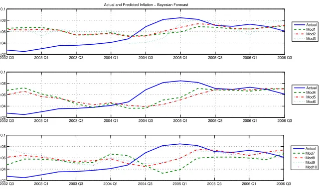
2002 Q3 2003 Q1 2003 Q3 2004 Q1 2004 Q3 2005 Q1 2005 Q3 2006 Q1 2006 Q3 0.02
0.04 0.06 0.08 0.1
Actual and Predicted Inflation − Bayesian Forecast
Actual Mod1 Mod2 Mod3
2002 Q3 2003 Q1 2003 Q3 2004 Q1 2004 Q3 2005 Q1 2005 Q3 2006 Q1 2006 Q3 0.02
0.04 0.06 0.08 0.1
Actual Mod4 Mod5 Mod6
2002 Q3 2003 Q1 2003 Q3 2004 Q1 2004 Q3 2005 Q1 2005 Q3 2006 Q1 2006 Q3 0.02
0.04 0.06 0.08 0.1
Actual Mod7 Mod8 Mod9 Mod10
[image:32.612.135.456.433.623.2]1988 Q1 1990 Q1 1992 Q1 1994 Q1 1996 Q1 1998 Q1 2000 Q1 2002 Q1 2004 Q1 2006 Q1 2008 Q1 −0.20
−0.15 −0.10 −0.05 0 0.05
0.10 0.15 0.2 0 0.25
Inflation Rate and Output Gap Estimates, 1989 Q4 − 2006 Q3
[image:33.612.144.440.297.483.2]Inflation Rate HP Gap CES Gap SVAR Gap