Proportional Integral Plus Control Strategy of an Intelligent Excavator

Proportional-Integral-Plus control

of an Intelligent Excavator

Jun Gu, C. James Taylor and Derek Seward Engineering Department,

Lancaster University, Lancaster, LA1 4YR, UK Email: [email protected]

Abstract—This paper considers the application of Proportional-Integral-Plus (PIP)

control to the Lancaster University Computerised Intelligent Excavator (LUCIE),

which is being developed to dig foundation trenches on a building site. Previous

work using LUCIE was based on the ubiquitous PI/PID control algorithm, tuned

on-line and implemented in a rather ad hoc manner. By contrast, the present

research utilises new hardware and advanced model-based control system design

methods to improve the joint control and so provide smoother, more accurate

movement of the excavator arm. In the paper, a novel nonlinear simulation model of

the system is developed for MATLAB/SIMULINK, allowing for straightforward

refinement of the control algorithm and initial evaluation. The PIP controller is

compared with a conventionally tuned PID algorithm, with the final designs

implemented on-line for the control of dipper angle. The simulated responses and

preliminary implementation results demonstrate the feasibility of the approach.

Keywords—Multivariable Control, True Digital Control, Proportional-Integral-Plus

I. INTRODUCTION

The civil and construction industries currently deploy a large number of manually controlled plants for a wide variety of tasks within the construction process. The excavation of foundations, general earthworks and earth removal tasks are activities which involve the machine operator in a series of repetitive operations. The automation of the earth removal process is likely to provide a number of benefits such as a reduced dependence on operator skills and a lower operator work load, both of which might be expected to contribute to improvements in quality. Automation also allows for the removal of the need for a human operator when working in hazardous environments.

In recent years there have been a number of papers concerned with the True Digital Control (TDC) design philosophy, in which the design of control systems is carried out overtly in discrete time. The foundations of the TDC approach are based upon the Simplified Refined Instrumental Variable (SRIV) identification and estimation algorithms for data-based modelling (Young, 1984; 1991), and the subsequent design of Proportional-Integral-Plus (PIP) control algorithms (e.g. Young et al., 1987; Chotai et al., 1998; Taylor et al., 2000a).

PIP controllers have been successfully designed for a range of difficult applications, including the control of CO2 in Open Top Chamber (OTC) and Free Air Carbon dioxide

Enrichment (FACE) systems (Lees et al., 1998; Taylor et al., 2000b); control of microclimate in horticultural glasshouses (Young et al., 1994); control of ventilation rate in animal houses and other agricultural buildings (Price et al., 1999); and the automatic positioning of an industrial piling rig system (Dixon et al., 1997).

The present paper considers the application of PIP control to the Lancaster University

developed to dig foundation trenches on a building site. LUCIE is based on a commercial manual hydraulic excavator, but has an on-board computer system in place of a driver to control the hydraulics and therefore the machine.

Previous work using LUCIE has demonstrated the feasibility of developing a machine that will dig a trench of specified dimensions (Bradley and Seward, 1998). To date, however, control of the excavator arm has been based on the ubiquitous PI/PID type control algorithms, tuned on-line and implemented in a rather ad hoc manner. By contrast, the present research utilises model-based PIP design to improve the joint control and so provide smoother, more accurate movement of the excavator arm. The ultimate aim is to develop a machine that will autonomously traverse a building site and dig a series of trenches without human intervention. In this regard, one advantage of PIP control is that it provides a rigorous approach for the estimation of the control parameters, which may be straightforwardly optimised for the different operating conditions encountered by the excavator arm, such as movement in the air and digging in soils of varying consistency.

Finally, it should be pointed out that the research takes full advantage of new hardware now built into LUCIE. For example, the approach proposed in this paper incorporates the inverse kinematics into the on-line controller, which has only become possible with the wide availability of more powerful on-line computing resources.

Fig.1. The LUCIE Excavator.

II. OVERVIEW of PIP CONTROL

• data-based identification and estimation of discrete-time, linear Transfer Function (TF) models, using the optimal Refined Instrumental Variable (RIV) or SRIV algorithms (Young 1984; 1991);

• PIP control system design using these estimated models (Young et al., 1987; 1994);

• initial evaluation of the design using computer simulation;

• real time implementation and evaluation of the controller.

For ease of presentation, the general multivariable PIP methodology is described below. However, it should be pointed out that in the preliminary results presented later, these equations are straightforwardly reduced to the single-input, single-output (SISO) case. Here, the transfer function model takes the following general form:

) ( ) ( ) ( ) ( 1 ) ( 1 1 1 1 1

1 _{u k}

z A z B k u z a z a z b z b k y n n m m − − − − − − = + + + + + = ⋯ ⋯ (1)

where A(z−1) and B(z−1) are appropriately defined polynomials in the backward shift operator z−1; i.e., z−iy(k)= y(k−i). For convenience, any pure time delay of δ>1 samples can be accounted for by setting the δ−1 leading parameters of the B(z−1) polynomial to zero, i.e. b₁…b_δ−1 =0_.

In the NMSS approach to control system design, the Transfer Functions (TF) are usually identified from measured input-output data, collected either from planned experiments or during the normal operation of the plant. In all cases, however, it is recommended that the required identification and estimation analysis should utilise the optimal Refined Instrumental Variable (RIV) or SRIV algorithms (Young, 1984; 1991) since they are often more robust to noise model specification in this regard than alternatives, such as the methods available in the MATLAB Identification Toolbox. For a given physical system, an appropriate model structure needs to be identified, i.e. the most appropriate values for the triad [n,m,δ] in equation (1) above. The two main statistical measures employed to help determine these values are the coefficient of determination R_T2, based on the response error, which is a simple measure of model fit; and the more sophisticated Young Identification Criterion (YIC), which provides a combined measure of fit and parametric efficiency, with large negative values indicating a model which explains the output data well, without over-parameterisation (Young, 1991). Note that these statistical tools and associated estimation algorithms have been assembled as the Captain toolbox within the MATLAB software environment (http://www.es.lancs.ac.uk/cres/systems.html). The second author can be contacted for further details about the toolbox, which is presently in the “beta” testing stage of its development.

implementation of any state variable feedback (SVF) design technique, for example: pole assignment or optimal linear quadratic (LQ) control, as discussed below.

A. The NMSS Form

Consider the following r-input, p-output, discrete time system represented in the terms of left Matrix Fraction Description (MFD) (Kailath, 1980).

) ( ) ( )] ( [ )

(k A z 1 1B z 1 u k

y = − − − (2) or, ) ( ) ( ) ( )

(z 1 y k B z 1 u k

A − = −

where, n n 1 1 1 ... ) ( )

(z− =I+A z− + +A z−

A (A_n ≠0)

m m 1 1 1 ... )

(z− =B z− + +B z−

B (B_m ≠0)

Here, A_i(i=1,2,…,n) are p×p matrices and B_i (i=1,2,…,m) are p×r matrices. If required, some of the initial B terms could take null values to accommodate pure time delays in the system. The state vector for the NMSS form is defined as,

] ) ( 1) m (k ... ) ( 1) ( ... 1) ( ) ( [ )

(k y k Ty k T y k n Tu T u Tz k T

x = − − + _k−₁ − + (3)

where the vectors y(k) and (k)u are, in this case, vectors of system outputs and control inputs. The integral-of –error vector z(k) is defined as,

1 d 1 )] ( ) ( [ ) ( ₋ − − z k k

k y y

associated with the relevant system output. Having defined the above state vector, the NMSS model can be formulated directly in the following form,

) ( 1) ( 1) ( )

(k Fx k Gu k Dy_d k

x = − + − + (5)

) ( )

(k Hx k

y = (6)

where F, G, D and H are formulated matrices:

                                  − − − − − − − − = − − − − p m m n n r r r p p p m m n n I B B B B A A A A I I I I I I B B B B A A A A F 1 3 2 1 2 1 1 3 2 1 2 1 0 0 0 0 0 0 0 0 0 0 0 0 0 0 0 0 0 0 0 0 0 0 0 0 0 0 0 0 0 0 0 0 0 0 0 0 0 0 0 0 0 0 0 0 0 0 0 0 0 0 0 0 0 0 0 0 0 0 ⋯ ⋯ ⋯ ⋮ ⋯ ⋮ ⋮ ⋮ ⋱ ⋮ ⋮ ⋮ ⋱ ⋮ ⋮ ⋯ ⋯ ⋯ ⋯ ⋯ ⋯ ⋯ ⋯ ⋮ ⋮ ⋮ ⋱ ⋮ ⋮ ⋮ ⋮ ⋱ ⋮ ⋮ ⋯ ⋯ ⋯ ⋯ ⋯ ⋯ (7) and,

[

]

1 r

1 0 0 ... 0 I 0 0 ... 0 B

B

G= − (8)

[

]

0 ... 0 0 0 0 ... 0 0

0 I_p

D= (9)

[

]

0

0 …

p

I

H= (10) Here, the block matrices I_p and Ir denote p× pand p×r identity matrices,

B. The PIP Control Law

The multivariable SVF control law is defined in the usual fashion, i.e., )

( )

(k Lx k

u =− (11)

or ) ( 1) ( 1)... ( 1) ( 1)... ( ) ( )

(k L₀y k L₁yk L_n1yk n M₁uk M_{m 1}uk m K_izk

u =− − − − ₋ − + − − − ₋ − + +

(12) where,

] ...

...

[L₀ L₁ L _{n 1} M ₁ M _{m 1} K _i

L = _{− −} −

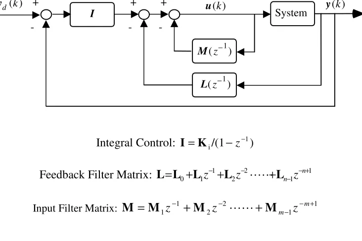
is the SVF control gain matrix. The general block diagram for the closed loop system is shown in Fig.2.

Fig. 2. Proportional-Integral-Plus (PIP) Control in Block Diagram Form.

C. Optimal PIP Linear Quadratic (PIP-LQ) Control

In the present research, the NMSS form is typically used as a foundation for the design of optimal PIP-LQ controllers. Here, the requirement is to design a control gain matrix L, which minimises the well-known linear quadratic performance criterion,

(

)

i Qx u Ru

x

J (13)

the elements of Q have a simple interpretation. That is, the diagonal elements portray the weights assigned to values of the input and output variables, and the integral-of-error terms.

The feedback gain matrix L which minimises the cost function J can be computed in a variety of ways; e.g. by means of the well-known iterative algorithm for computing the steady state solution of the associated, discrete time Riccati equation (Kleinman, 1974), given the NMSS system description [F, G] and the weighting matrices (Q, R).

III. LUCIE and PROBLEM DEFINITION

In recent years, the Engineering Department at Lancaster University has combined the three disciplines of civil, mechanical and electrical engineering into one “Mechatronic” project — the Lancaster University Computerised Intelligent Excavator (LUCIE). Based on a commercial manual hydraulic excavator, LUCIE has an on-board computer system to control the hydraulics. It is being developed with one particular task in mind: the digging of foundation trenches on a building site. The ultimate aim is to develop a machine that will be able to accept a program of trench locations and dimensions and then traverse a building site and dig a series of trenches meeting these specifications. It should do this autonomously without human intervention.

A. System Architecture:

1.The movement of the arm in an (x, y) vertical plane, using two hydraulic cylinders which control the boom and dipper respectively.

2.The rotation of the bucket at the end of the dipper, in the same vertical plane, using another cylinder.

3.The rotation of the cab at its connection to the undercarriage, effectively providing movement for the arm in a horizontal plane (slew).

4.The movement up and down of a dozer blade at the front of undercarriage.

5.The movement of two parallel caterpillar tracks independently, backwards and forwards.

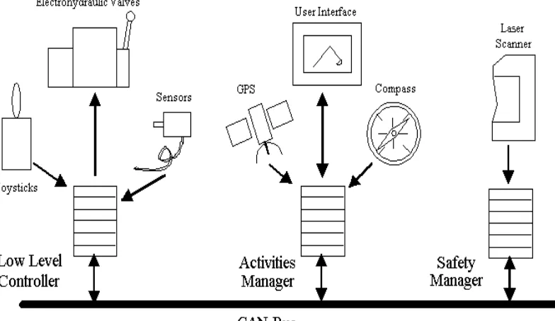
The excavator is automated by installing a distributed computer architecture to control its hydraulics and, therefore, all the movements. As shown by Fig. 3, the "Brain" of the excavator relies on three embedded PC104 computers, each computer being responsible for a separate task. Communication between the computers is provided by the CAN-Bus (Controller Area Network) a robust communications protocol developed within the automotive industry.

Fig.3. Hardware Architecture for Excavator Control.

• An activities manager (AM) is responsible for issuing high-level commands for digging and navigation. This contains the knowledge base extracted from theoretical studies and the experiences of actual expert operators.

• The safety manager (SM) operates as the excavator supervisor ensuring that the machine remains in a safe stable condition.

The sensory equipment is summarised below:

• Four potentiometers on the joints for angle measurement.

• A two-axis tilt sensor.

• A Leuze RotoScan RS 3 optical laser distance sensor, for obstacle detection up to a range of 15 m.

• A Trimble 7400Msi series satellite GPS for location and navigation.

B. Operation and High Level Control Strategy:

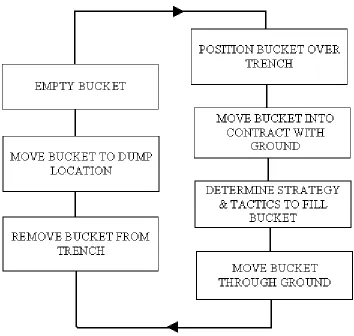
The first, and only fully predictable, action of the LUCIE system is to extend the arm to its fullest extent and then lower it until the tip of the bucket contacts the ground (Bradley and Seward, 1998). Once the ground, which is the start-point of excavating, has been detected, the excavator attempts to penetrate the ground to a point at which the bucket can be filled by rotation. If this is not possible, because the ground is too hard, the bucket is scraped towards the cab in a dragging motion in order to loosen enough material to fill the bucket. The arm is then slewed to deposit the earth and finally returned to the previous point of entry to start another cycle. During this procedure, the system remembers the previous point of entry into the ground and the swept profile. This is then compared with the desired profile. At the end of the process, a trench is produced. The sequence of operation (Bradley and Seward, 1998) is defined by Fig .4.

During excavation it is sometimes necessary for the trajectory of the tip of the bucket to be a straight line. For example, when LUCIE is dragging in the ground in order to complete a flat bottomed trench, the trajectory of the bucket is a straight horizontal line. The overall control requirements can therefore be summarised as:

1. The ability to move the teeth of the excavator bucket from point-to-point through a specified trajectory.

2. The need to adapt the digging strategy in order to fill the bucket in the minimum cycle time. This implies the need to provide the activities manager with adequate progress data so that strategic decisions can be made.

It can be seen that during the whole operation, the proper and precise position of each joint of LUCIE is an essential requirement if it is to carry out its designed task. It is clear that the high level controller, which decides the overall excavation strategy, depends on fast robust regulation of these low level variables, as considered in the following section IV of the paper.

IV. PIP CONTROL SYSTEM DESIGN

A. PIP control of bucket position

This research combines the previously developed kinematics (Bradley and Seward, 1998) with TF models for the joint dynamics obtained from experimental data, in order to develop a nonlinear simulation model for LUCIE. The simulation is utilised to demonstrate the proposed PIP control methodology and identify the limitations of conventional PID design.

A.1. Dipper and Boom Kinematics

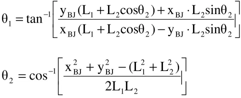
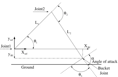
Assuming minimal flexure in the boom and dipper arms, the fixed geometry of the system ensures a static relationship between the joint angles and the (x,y) coordinates for the reference point on the bucket. As shown in Fig. 5, the reference (0, 0) point for the coordinate system used in the kinematic analysis is the point of attachment of the boom to the vehicle, with positive motion in the x-direction being away from the vehicle and positive motion in the y-direction being vertically upwards. During digging, referring again to Fig. 5, the position of bucket joint (xBJ,yBJ) relative to the

reference point is obtained from the following equations (Bradley and Seward, 1998): )

( 1 2 2

1 1

BJ L cosθ L cos θ θ

x = + − (14) )

( 1 2 2

1 1

BJ L sinθ L sin θ θ













⋅

−

+

⋅

+

+

=

sin

θ

L

y

)

cos

θ

L

(L

x

sin

θ

L

x

)

cos

θ

L

(L

y

tan

θ













₊

₋

₊

=

L

2L

)

L

(L

y

x

cos

θ

Fig.5. Excavator Kinematics.

A.2. Data-Based Models for the Joint Dynamics

In the present section, discrete-time, linear models of the joint dynamics are estimated from experimental data using the SRIV algorithm (Young, 1991). For example, Fig. 6 shows the response of the boom, from an initial closed position, to a series of input voltages ranging from 100 to 900 (scaled units: see later). In each case, the boom opens at a speed proportional to the input voltage until it reaches it’s maximum extended position, typically 2-3 seconds later. In Fig. 6, the initial boom angle is approximately 10 degrees; however, the data are stacked for clarity of presentation, with the traces higher up the plot representing experiments with larger input voltages.

Fig. 6. Boom Opening Response for Different Drive Demands (dots) and Estimated TF Model (solid).

degrees, where the later figure represents fully open. Similarly, a scaled input voltage to the dipper in the range -1000 to 1000 causes the dipper angle to vary from -30 (fully open) to -140 degrees. The hydraulic pressure that drives the arms is approximately 1.1×107 pa. Finally, all the modelling and control design is based on a sampling rate of 0.1 seconds, which is within the capabilities of the on-line computer and is found to work well in practice.

In common with other hydraulic systems (e.g. Dixon et al., 1997), it is clear that the boom angle behaves as an integrator, with an almost constant rate of change for a given input signal (see Fig. 6). This is confirmed by a model identification exercise utilising R_T2 and YIC, where the transfer function model is each case is found to be of the following first order form:

( )

1 ) (

1 1

k u z z b k y

− −

−

= (18)

Here, y(k) represents the boom angle, u(k) the input voltage and b is a numerator parameter estimated for each experiment in turn. It is important to stress that the linear model (18) is based on a time invariant parameter b and, therefore, only holds for a specified input voltage. For example, when u(k)=500, then the SRIV algorithm determines that b=0.0029 and R_T2 =0.9986, i.e. over 99% of the variation in the data is explained by the simple TF model (18). Indeed, as illustrated in Fig. 6, the response of the model (solid trace) closely matches the data (dots) for each experiment.

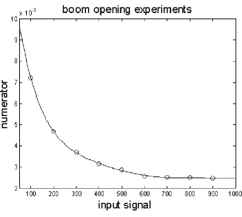
Fig. 7. Numerator Parameter b for Equation (18) Fitted to Experimental Boom Opening Data, Plotted against the Input Voltage (dots); Estimated Curve (solid).

Experiments utilising negative voltages to close the boom reveal a similar, albeit inverted, series of responses to Fig. 6. However, in this case, the R_T2 and YIC criteria suggest that the most appropriate model structure has two samples pure time delay, i.e.,

( )

1 ) (

1 2

k u z z b k y

− −

−

= (19)

In this case, the relationship between b and the input voltage can also be fitted with a 6th order polynomial. Therefore, by combining Fig. 7 and the equivalent curve for the boom closing experiments, with the transfer function models (18) and (19), the dynamic relationship between boom angle and any specified input voltage may be determined.

Furthermore, similar TF models may be obtained for dipper opening and dipper closing experiments, here with unity pure time delays for both cases. In this manner, a nonlinear simulation model is developed for LUCIE and implemented using MATLAB/SIMULINK as illustrated in Fig. 8. The model is based on the following three components:

• The simulation inputs are the applied voltages to the boom and dipper joints. In SIMULINK, a switch determines whether the joint is opening or closing and the appropriate parameter b is determined from the previously estimated nonlinear curve, such as Fig. 7.

• These joint angles are utilised to determine the bucket position from the kinematic equations (14) and (15), yielding the simulation output in the form of (x_BJ,y_BJ) coordinates (cm).

A.3. PIP control system design

The specifications for the movement of bucket position in a straight line are as follows.

• When the bucket moves in the air, the trajectory should keep an accuracy of

±100mm

• When it moves in the ground, the accuracy should be kept to within ±25mm. Cycle times are also a major factor in determining performance. Observation of machine operators on this size of excavator suggest that a typical cycle time, for an average operator completing the sequence of operations defined by Fig. 4, is of the order of 15 to 25 seconds depending on the type of ground. The operation of moving the bucket through the ground is typically between 5 to 8 seconds.

As will become apparent, these two TF models and associated fixed gain PIP control algorithms, yield good control of the bucket when applied to the full nonlinear simulation. Indeed, straightforward tuning quickly yields PIP-LQ controllers for the boom and dipper angles: the results discussed below are based on unity weights for the input and output states, together with weightings of 10 for the integral of error states.

Fig. 8 shows the SIMULINK implementation of the nonlinear model, together with the associated PIP control algorithm. Here, the two subgroups shown in the top level diagram are illustrated below in Fig. 8 (b) and (c). For brevity, further levels of complexity are not shown in the figure – for example, the “Digger Geometry” subgroup in Fig. 8 (b) contains the kinematic equations (14) and (15), which are programmed in SIMULINK using Switches and MATLAB functions.

(a) Top Level Diagram. (b) PIP Control Subgroup. (c) LUCIE Simulation Subgroup.

Fig.8. SIMULINK Diagram For the Bucket Position Control System.

In this formulation, the desired (x, y) coordinates for bucket position are fed into the inverse digger geometry algorithm, represented as one of the subgroups in Fig. 8 (b). Here the equivalent joint angles are calculated from equations (16) and (17). These angles provide the set points for the PIP control systems. One PIP control algorithm utilises the boom voltage to control the boom angle, while a second utilises the dipper voltage to control the dipper angle.

disturbances influencing the (x, y) coordinates or their rate of change, such as the bucket hitting a rock, will still be fed back to the control algorithm through their inherent affect on the measured joint angles. The advantage of concentrating on the joint angles in this way, is that the nonlinear digger geometry is accounted for at the design stage whilst, since there is a clearly established instantaneous relationship between joint angles and the (x, y) coordinates, no useful control information is lost. Furthermore, this approach can be employed for both movement of bucket in the air and in the ground for digging.

A typical closed loop experiment would consist of moving the bucket from position (x1,y1) to (x2,y2). The specified trajectory could take the form of a straight line or could

be curved, and may have either constant or time varying speed. Ultimately, the trajectory chosen will depend on the nature of the trench being dug and could be revised on-line by a high level control system.

A.4. PIP control system evaluation and comparison with PID control

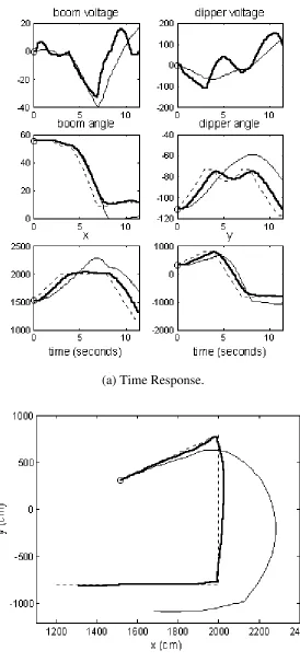
To illustrate the proposed control scheme, consider the simulation response shown in the time series and polar coordinate plots of Fig. 9 (a) and Fig. 9 (b) respectively. The objective of this simulation experiment is to move the bucket from its initial position {1500, 300}, to {2000, 800}, {2000, -800} and {1200, -800}, where the {x, y} coordinates are given in cm from the reference point. The trajectory between each set of coordinates should take the form of a straight line and be complete in 3 seconds, with a wait of 1 second at each location.

the joint angle set points calculated on-line, shown as dashed traces in the middle two plots of Fig. 9 (a), and the PIP control algorithms adjusting the input voltage (top graphs) in order to meet these targets. It is clear from Fig. 9 (b) that the bucket is moved along the defined straight-line trajectories well within the required accuracy (thick trace).

(a) Time response. (b) Polar coordinate plot.

Fig. 9. Nonlinear Simulation of Bucket Movement, Comparing PIP (thick), PID (thin) and Set Points (dashed).

Fig. 9 also shows the response of a carefully tuned PID algorithm applied to the same nonlinear simulation. The PID algorithm was obtained using the Ziegler-Nichols ultimate sensitivity method (Franklin et al., 1994), followed by extensive subsequent experimental tuning. For this simulation example, it is clear that PID control does not meet the performance requirements.

Previous research has shown it is possible, under certain conditions, to control the individual joints of LUCIE using PI/PID type algorithms. Indeed, by using a system of ad hoc rules, Bradley and Seward (1998) obtain reasonable, albeit sometimes juddering, control of the bucket. However, the present formulation of the control problem, using the kinematics to resolve the motion, requires fast precise regulation of the joint positions and this not always possible using conventionally tuned PID algorithms. Examination of Fig. 9 reveals that small errors in the joint angles lead to large mismatches in the final bucket position.

reason why the authors have turned to the more sophisticated PIP approach, which is able to handle time delays automatically (Taylor et al., 1998).

B. Dipper Angle On-Line Implementation

The present section discusses on-line results concentrating on control of the dipper angle. To the authors knowledge, this is the first time PIP control has been applied to such a heavy excavator, and these preliminary experiments are designed to assess the feasibility of the approach.

B.1. Dipper Angle Control System Design and Implementation

Based on a dipper closing experiment with an input voltage of –600, a first order TF model with unity time delay is identified (R2_T=0.99927 and YIC=-17.63) and utilised in the design of the following PIP control algorithm:

) ( 6.8θ 1) θ₍ 74.8θ 1)

u( )

u(k = k− + (k)- k− − d k (20)

where θ ( )

d k is the set point for the dipper angle at sample k.

In the frequency domain, the conservative gain and phase margins were calculated at Gm=10.0083dB and Pm=180 . These values are well within the acceptable bounds. For o example, a typical aerospace application might specify margins of 4dB and

36

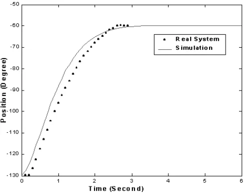
The results are shown in Fig. 10, where it can be seen that the dipper reaches its target angle in about 2 or 3 seconds.

(a) Set point step from -130 to -60 degrees. (b) Set point step from -130 to -40 degrees. (c) Set point step from -60 to -110 degrees.

Fig. 10. PIP Control of LUCIE Dipper Angle Compared with Response of Linear TF model.

B.2. Analysis and Evaluation

The results illustrated in Fig. 10 suggest that the PIP control system satisfies the requirement of driving the arm to the target angle in a fast and smooth manner. However, a number of avenues for improvement have been identified and are discussed below:

• For simplicity, an integrator with unity time delay is assumed for the TF model. However, this is not necessary the most appropriate model structure for control of the dipper. The authors are presently investigating the applicability of a 2nd order double integrator model, possibly with two or more time delays.

• The TF models used in the control designs above are all based on a single input voltage to either the dipper or boom, yielding fixed gain PIP controllers that are particularly simple to implement. However, in practice, it is clear that different input voltages yield different responses, as shown in Fig. 6. One simple improvement would be to utilise different control models for the opening and closing cases. At the other extreme, it may prove beneficial to implement a fully scheduled PIP controller, where the control parameters are updated at each sample by determining the b parameter from a previously estimated curve such as Fig. 7.

• Finally, the authors are presently investigating the application of multi-objective optimisation techniques (Chotai et al., 1998) in order to account for some of the above practical limitations. PIP control is ideal for incorporation within such as framework, where satisfactory compromise can be obtained between conflicting objectives such as robustness, overshoot, rise times and multivariable decoupling. This is achieved by concurrent optimisation of the diagonal and off diagonal elements of the weighting matrices in the cost function. Since it is the LQ weights that are optimised, this has the advantage of generating only guaranteed stable optimal solutions, thus allowing for better (smoother) defined optimisation problems. This is one advantage of utilising a model-based approach such as PIP, rather than attempting to directly tuning the gains of a PID type algorithm.

V. CONCLUSION

factors that must be considered, including the affect of gravity, hydraulic pressure, inertia during motion, time delays and the uncertain working environment. These represent the huge challenges for the automatic control of the LUCIE excavator.

Previous attempts to control LUCIE have yielded relatively slow and sometimes juddering responses. The present work aims to improve the speed and smoothness of bucket control by utilising new hardware and advanced model-based control methods. In particular, this paper proposes a bucket position controller for LUCIE that couples the inverse kinematic equations with high performance Proportional-Integral-Plus (PIP) controllers for the joint angles.

The authors are presently investigating the application of multi-objective optimisation techniques, in order to further improve the performance of the joint controllers, before evaluating the proposed bucket control system on-line. This research will be reported in future publications. However, the simulated responses discussed above, together with the preliminary implementation results, are very promising.

ACKNOWLEDGEMENTS

The authors are grateful to the UK Engineering and Physical Sciences Research Council (EPSRC), Overseas Research Students Awards Scheme (ORS), The Institution of Electrical Engineers (IEE) and Peel Studentship Trust Fund for supporting this research; to the Nuffield Foundation for their support of the second author.

REFERENCES

Bradley D.A. and Seward D.W. (1998). The Development, Control and Operation of an

Chotai, A., Young, P.C., Mckenna, P.G. and Tych, W. (1998). Proportional-Integral-Plus (PIP) design for delta (δ) operator systems: Part 2, MIMO systems, Int. J. Control, 70, 149-168.

Dixon R., Chotai A., Young P.C. and Scott J.N. (1997). The Automation of Piling Rig

Positioning Utilising Multivariable Proportional-Integral-Plus (PIP) Control, Proc. 12th Int. Conf. on Systems Engineering, ICSE’97, Coventry University, UK, 9-11 September.

Franklin, G.F., Powell, J.D. and Emami-Naeini, A. (1994). Feedback control of

dynamic systems, Addison Wesley (3rd Ed.).

Kailath, T. (1980). Linear Systems, prentice-Hall, Englewood Cliffs, N.J..

Kleinman D.L. (1974). Stabilizing a Discrete, Constant, Linear System with Application

to Iterative Methods for Solving the Riccati Equation, IEEE Trans., Vol.AC-19. Lees, M.J., Taylor, C.J., Young, P.C. and Chotai, A. (1998). Modelling and PIP

control design for Open Top Chambers, Control Engineering Practice, 6, 1209-1216. Price, L., Young, P., Berckmans, D., Janssens, K.and Taylor, J. (1999). Data-Based

Mechanistic Modelling (DBM) and Control of Mass and Energy transfer in agricultural buildings, Annual Reviews in Control, 23, 71-82.

Taylor, C.J., Chotai, A. and Young, P.C. (1998), Proportional-Integral-Plus (PIP)

control of time delay systems, Proceedings of the Institution of Mechanical Engineers, Journal of Systems and Control Engineering, 212, Part I, 37-48.

Taylor, C.J., Chotai, A. and Young P.C. (2000a). State space control system design

based on non-minimal state-variable feedback: Further generalisation and unification results, International Journal of Control, 73, 1329-1345.

Taylor, C.J., Young, P.C. Chotai A., Mcleod, A.R. and A.R. Glasock (2000b).

Modelling and Proportional-Integral-Plus Control Design for Free Air Carbon Dioxide Enrichment systems, Journal of Agricultural Engineering Research, 75, 365-374.

Young, P.C. (1984). Recursive Estimation and Time Series Analysis (Communication

Young, P.C. (1991). Simplified Refined Instrumental Variable (SRIV) estimation and

True Digital Control (TDC): a tutorial introduction, Proceedings of the First European Control Conference, Grenoble.

Young P.C., Behzadi M.A., Wang C.L. and Chotai A. (1987). Direct Digital and

Adaptive Control by Input-Output, State Variable Feedback Pole Assignment, International Journal of Control, 46.

Young P.C., Lees M.J., Chotai A., Tych W. and Chalabi Z.S. (1994). Modelling and

1370mm

1

5

0

0

m

m

7

2

0

m

m

Potentiometer4

Potentiometer1 Potentiometer3

Potentiometer2

Dipper

Bucket Boom

3 5

4

1

2

System

M(z−1)

L(z−1)

I y(k)

y_d(k) + _u(k)

-+

-+

-Integral Control: I=K_i/(1−z−1)

Feedback Filter Matrix: = ₀+ ₁ −1+ ₂ −2 + ₋₁ −n+1 n z z

z L L

L L

L ⋯⋯

Input Filter Matrix: M =M₁z−1+M₂z−2⋯⋯+M_m−1z−m+1

Joint1

Joint2

Bucket

Joint

Ground

Angle of attack

ref

X

ref

y

BJ

X

1

L

1

θ

α

2

θ

2

L

BJ

y

3

θ

(a) Top Level Diagram.

(b) PIP Control Subgroup

(c) LUCIE Simulation Subgroup.

(a) Time Response.

(b) Polar Coordinate Plot.

(a) Set point step from -130 to -60 degrees.

(b) Set point step from -130 to -40 degrees.