Essential guidelines for computational method benchmarking

R E V I E W

Open Access

Essential guidelines for computational

method benchmarking

Lukas M. Weber

, Wouter Saelens

, Robrecht Cannoodt

, Charlotte Soneson

, Alexander Hapfelmeier

,

Paul P. Gardner

, Anne-Laure Boulesteix

, Yvan Saeys

and Mark D. Robinson

Abstract

In computational biology and other sciences, researchers are frequently faced with a choice between several computational methods for performing data analyses. Benchmarking studies aim to rigorously compare the performance of different methods using well-characterized benchmark datasets, to determine the strengths of each method or to provide recommendations regarding suitable choices of methods for an analysis. However, benchmarking studies must be carefully designed and implemented to provide accurate, unbiased, and informative results. Here, we summarize key practical guidelines and recommendations for performing high-quality benchmarking analyses, based on our experiences in computational biology.

Introduction

Many fields of computational research are characterized by a growing number of available methods for data ana-lysis. For example, at the time of writing, almost 400 methods are available for analyzing data from single-cell

RNA-sequencing experiments [1]. For experimental

re-searchers and method users, this represents both an op-portunity and a challenge, since method choice can significantly affect conclusions.

Benchmarking studies are carried out by computa-tional researchers to compare the performance of differ-ent methods, using reference datasets and a range of evaluation criteria. Benchmarks may be performed by authors of new methods to demonstrate performance improvements or other advantages; by independent groups interested in systematically comparing existing

methods; or organized as community challenges. ‘

Neu-tral’ benchmarking studies, i.e., those performed inde-pendently of new method development by authors without any perceived bias, and with a focus on the comparison itself, are especially valuable for the research community [2,3].

From our experience conducting benchmarking stud-ies in computational biology, we have learned several key lessons that we aim to synthesize in this review. A number of previous reviews have addressed this topic from a range of perspectives, including: overall

commen-taries and recommendations on benchmarking design [2,

4–9]; surveys of design practices followed by existing

benchmarks [7]; the importance of neutral

benchmark-ing studies [3]; principles for the design of real-data

benchmarking studies [10, 11] and simulation studies

[12]; the incorporation of meta-analysis techniques into

benchmarking [13–16]; the organization and role of

community challenges [17, 18]; and discussions on

benchmarking design for specific types of methods [19,

20]. More generally, benchmarking may be viewed as a

form of meta-research [21].

Our aim is to complement previous reviews by provid-ing a summary of essential guidelines for designprovid-ing,

per-forming, and interpreting benchmarks. While all

guidelines are essential for a truly excellent benchmark, some are more fundamental than others. Our target audience consists of computational researchers who are interested in performing a benchmarking study, or who have already begun one. Our review spans the full ‘

pipe-line’ of benchmarking, from defining the scope to best

practices for reproducibility. This includes crucial ques-tions regarding design and evaluation principles: for ex-ample, using rankings according to evaluation metrics to

© The Author(s). 2019Open AccessThis article is distributed under the terms of the Creative Commons Attribution 4.0 International License (http://creativecommons.org/licenses/by/4.0/), which permits unrestricted use, distribution, and reproduction in any medium, provided you give appropriate credit to the original author(s) and the source, provide a link to the Creative Commons license, and indicate if changes were made. The Creative Commons Public Domain Dedication waiver (http://creativecommons.org/publicdomain/zero/1.0/) applies to the data made available in this article, unless otherwise stated.

* Correspondence:yvan.saeys@ugent.be;mark.robinson@imls.uzh.ch 3

Data Mining and Modelling for Biomedicine, VIB Center for Inflammation Research, 9052 Ghent, Belgium

1_{Institute of Molecular Life Sciences, University of Zurich, 8057 Zurich,}

Switzerland

identify a set of high-performing methods, and then highlighting different strengths and tradeoffs among these.

The review is structured as a series of guidelines (Fig. 1), each explained in detail in the following sec-tions. We use examples from computational biology; however, we expect that most arguments apply equally to other fields. We hope that these guidelines will con-tinue the discussion on benchmarking design, as well as assisting computational researchers to design and imple-ment rigorous, informative, and unbiased benchmarking analyses.

Defining the purpose and scope

The purpose and scope of a benchmark should be clearly defined at the beginning of the study, and will fundamentally guide the design and implementation. In general, we can de-fine three broad types of benchmarking studies: (i) those by method developers, to demonstrate the merits of their ap-proach (e.g., [22–26]); (ii) neutral studies performed to sys-tematically compare methods for a certain analysis, either conducted directly by an independent group (e.g., [27–38]) or in collaboration with method authors (e.g., [39]); or (iii) those organized in the form of a community challenge, such as those from the DREAM [40–44], FlowCAP [45, 46], CASP [47,48], CAMI [49], Assemblathon [50,51], MAQC/ SEQC [52–54], and GA4GH [55] consortia.

A neutral benchmark or community challenge should be as comprehensive as possible, although for any bench-mark there will be tradeoffs in terms of available re-sources. To minimize perceived bias, a research group conducting a neutral benchmark should be approximately equally familiar with all included methods, reflecting

typical usage of the methods by independent researchers [3]. Alternatively, the group could include the original method authors, so that each method is evaluated under optimal conditions; methods whose authors decline to take part should be reported. In either case, bias due to fo-cusing attention on particular methods should be

avoided—for example, when tuning parameters or fixing

bugs. Strategies to avoid these types of biases, such as the use of blinding, have been previously proposed [10].

By contrast, when introducing a new method, the focus of the benchmark will be on evaluating the relative merits of the new method. This may be sufficiently achieved with a less extensive benchmark, e.g., by comparing against a smaller set of state-of-the-art and baseline methods. How-ever, the benchmark must still be carefully designed to avoid disadvantaging any methods; for example, exten-sively tuning parameters for the new method while using default parameters for competing methods would result in a biased representation. Some advantages of a new method may fall outside the scope of a benchmark; for ex-ample, a new method may enable more flexible analyses than previous methods (e.g., beyond two-group compari-sons in differential analyses [22]).

Finally, results should be summarized in the context of the original purpose of the benchmark. A neutral bench-mark or community challenge should provide clear guidelines for method users, and highlight weaknesses in current methods so that these can be addressed by method developers. On the other hand, benchmarks per-formed to introduce a new method should discuss what the new method offers compared with the current state-of-the-art, such as discoveries that would otherwise not be possible.

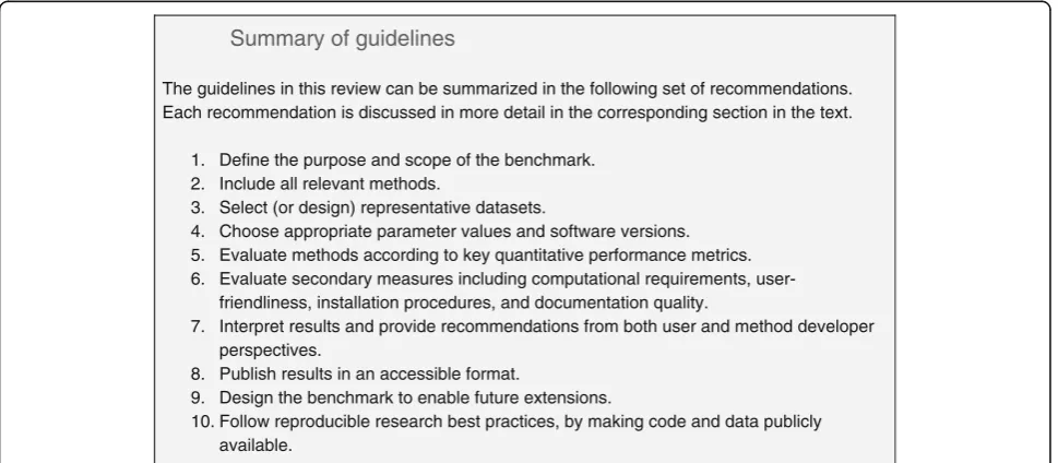
Summary of guidelines

The guidelines in this review can be summarized in the following set of recommendations. Each recommendation is discussed in more detail in the corresponding section in the text.

1. Define the purpose and scope of the benchmark. 2. Include all relevant methods.

3. Select (or design) representative datasets.

4. Choose appropriate parameter values and software versions. 5. Evaluate methods according to key quantitative performance metrics. 6. Evaluate secondary measures including computational requirements,

user-friendliness, installation procedures, and documentation quality.

7. Interpret results and provide recommendations from both user and method developer perspectives.

8. Publish results in an accessible format.

9. Design the benchmark to enable future extensions.

10. Follow reproducible research best practices, by making code and data publicly available.

Selection of methods

The selection of methods to include in the benchmark will be guided by the purpose and scope of the study. A neutral benchmark should include all available methods for a certain type of analysis. In this case, the publica-tion describing the benchmark will also funcpublica-tion as a review of the literature; a summary table describing the methods is a key output (e.g., Fig. 2 in [27] or Table 1

in [31]). Alternatively, it may make sense to include

only a subset of methods, by defining inclusion criteria: for example, all methods that (i) provide freely available software implementations, (ii) are available for com-monly used operating systems, and (iii) can successfully be installed without errors following a reasonable amount of trouble-shooting. Such criteria should be chosen without favoring any methods, and exclusion of any widely used methods should be justified. A useful strategy can be to involve method authors within the process, since they may provide additional details on optimal usage. In addition, community involvement can lead to new collaborations and inspire future method development. However, the overall neutrality and

balance of the resulting research team should be main-tained. Finally, if the benchmark is organized as a com-munity challenge, the selection of methods will be determined by the participants. In this case, it is

im-portant to communicate the initiative widely—for

example, through an established network such as DREAM challenges. However, some authors may choose not to participate; a summary table document-ing non-included methods should be provided in this case.

When developing a new method, it is generally sufficient to select a representative subset of existing methods to compare against. For example, this could consist of the current best-performing methods (if known), a simple

‘baseline’method, and any methods that are widely used. The selection of competing methods should ensure an ac-curate and unbiased assessment of the relative merits of the new approach, compared with the current state-of-the-art. In fast-moving fields, for a truly excellent bench-mark, method developers should be prepared to update their benchmarks or design them to easily allow exten-sions as new methods emerge.

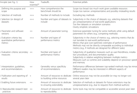
Table 1Summary of our views regarding‘how essential’each principle is for a truly excellent benchmark, along with examples of

key tradeoffs and potential pitfalls relating to each principle

Principle (see Fig.1) How

essential?a Tradeoffs Potential pitfalls

1. Defining the purpose and scope

+++ How comprehensive the benchmark should be

Scope too broad: too much work given available resources Scope too narrow: unrepresentative and possibly misleading results

2. Selection of methods +++ Number of methods to include Excluding key methods

3. Selection (or design) of datasets

+++ Number and types of datasets to include

Subjectivity in the choice of datasets: e.g., selecting datasets that are unrepresentative of real-world applications

Too few datasets or simulation scenarios Overly simplistic simulations

4. Parameter and software versions

++ Amount of parameter tuning Extensive parameter tuning for some methods while using default parameters for others (e.g., competing methods)

5. Evaluation criteria: key quantitative performance metrics

+++ Number and types of performance metrics

Subjectivity in the choice of metrics: e.g., selecting metrics that do not translate to real-world performance

Metrics that give over-optimistic estimates of performance Methods may not be directly comparable according to individual metrics (e.g., if methods are designed for different tasks)

6. Evaluation criteria: secondary measures

++ Number and types of performance metrics

Subjectivity of qualitative measures such as user-friendliness, installa-tion procedures, and documentainstalla-tion quality

Subjectivity in relative weighting between multiple metrics

Measures such as runtime and scalability depend on processor speed and memory

7. Interpretation, guidelines, and recommendations

++ Generality versus specificity of recommendations

Performance differences between top-ranked methods may be minor Different readers may be interested in different aspects of

performance

8. Publication and reporting of results

+ Amount of resources to dedicate to building online resources

Online resources may not be accessible (or may no longer run) several years later

9. Enabling future extensions ++ Amount of resources to dedicate to ensuring extensibility

Selection of methods or datasets for future extensions may be unrepresentative (e.g., due to requests from method authors)

10. Reproducible research best practices

++ Amount of resources to dedicate to reproducibility

Some tools may not be compatible or accessible several years later

a

Selection (or design) of datasets

The selection of reference datasets is a critical design choice. If suitable publicly accessible datasets cannot be found, they will need to be generated or constructed, either experimentally or by simulation. Including a variety of data-sets ensures that methods can be evaluated under a wide range of conditions. In general, reference datasets can be grouped into two main categories: simulated (or synthetic) and real (or experimental).

Simulated data have the advantage that a known true signal (or ‘ground truth’) can easily be introduced; for example, whether a gene is differentially expressed. Quantitative performance metrics measuring the ability to recover the known truth can then be calculated. How-ever, it is important to demonstrate that simulations accurately reflect relevant properties of real data, by inspecting empirical summaries of both simulated and real datasets (e.g., using automated tools [57]). The set of empirical summaries to use is context-specific; for ex-ample, for single-cell RNA-sequencing, dropout profiles and dispersion-mean relationships should be compared

[29]; for DNA methylation, correlation patterns among

neighboring CpG sites should be investigated [58]; for comparing mapping algorithms, error profiles of the

se-quencing platforms should be considered [59].

Simpli-fied simulations can also be useful, to evaluate a new method under a basic scenario, or to systematically test aspects such as scalability and stability. However, overly simplistic simulations should be avoided, since these will not provide useful information on performance. A fur-ther advantage of simulated data is that it is possible to generate as much data as required; for example, to study variability and draw statistically valid conclusions.

Experimental data often do not contain a ground truth, making it difficult to calculate performance met-rics. Instead, methods may be evaluated by comparing them against each other (e.g., overlap between sets of detected differential features [23]), or against a current widely accepted method or ‘gold standard’ (e.g., manual gating to define cell populations in high-dimensional cy-tometry [31,45], or fluorescence in situ hybridization to validate absolute copy number predictions [6]). In the context of supervised learning, the response variable to be predicted is known in the manually labeled training and test data. However, individual datasets should not be overused, and using the same dataset for both method development and evaluation should be avoided, due to the risk of overfitting and overly optimistic results [60,

61]. In some cases, it is also possible to design experi-mental datasets containing a ground truth. Examples in-clude: (i)‘spiking in’synthetic RNA molecules at known relative concentrations [62] in RNA-sequencing experi-ments (e.g., [54, 63]), (ii) large-scale validation of gene expression measurements by quantitative polymerase

chain reaction (e.g., [54]), (iii) using genes located on sex chromosomes as a proxy for silencing of DNA methyla-tion status (e.g., [26, 64]), (iv) using fluorescence-activated cell sorting to sort cells into known subpopula-tions prior to single-cell RNA-sequencing (e.g., [29, 65,

66]), or (v) mixing different cell lines to create‘ pseudo-cells’[67]. However, it may be difficult to ensure that the ground truth represents an appropriate level of variabil-ity—for example, the variability of spiked-in material, or whether method performance on cell line data is rele-vant to outbred populations. Alternatively, experimental datasets may be evaluated qualitatively, for example, by judging whether each method can recover previous dis-coveries, although this strategy relies on the validity of previous results.

A further technique is to design‘semi-simulated’

data-sets that combine real experimental data with an ‘in

silico’ (i.e., computational) spike-in signal; for example, by combining cells or genes from ‘null’ (e.g., healthy) samples with a subset of cells or genes from samples ex-pected to contain a true differential signal (examples in-clude [22,68,69]). This strategy can create datasets with more realistic levels of variability and correlation, to-gether with a ground truth.

Overall, there is no perfect reference dataset, and the selection of appropriate datasets will involve tradeoffs, e.g., regarding the level of complexity. Both simulated and experimental data should not be too ‘simple’ (e.g.,

two of the datasets in the FlowCAP-II challenge [45]

gave perfect performance for several algorithms) or too

‘difficult’(e.g., for the third dataset in FlowCAP-II, no al-gorithms performed well); in these situations, it can be impossible to distinguish performance. In some cases, individual datasets have also been found to be unrepre-sentative, leading to over-optimistic or otherwise biased assessment of methods (e.g., [70]). Overall, the key to truly excellent benchmarking is diversity of evaluations, i.e., using a range of metrics and datasets that span the range of those that might be encountered in practice, so that performance estimates can be credibly extrapolated.

Parameters and software versions

There are three major strategies for choosing parame-ters. The first (and simplest) is to use default values for all parameters. Default parameters may be adequate for many methods, although this is difficult to judge in ad-vance. While this strategy may be viewed as too simplis-tic for some neutral benchmarks, it reflects typical usage. We used default parameters in several neutral benchmarks where we were interested in performance for untrained users [27,71,72]. In addition, for [27], due to the large number of methods and datasets, total run-time was already around a week using 192 processor cores, necessitating judgment in the scope of parameter tuning. The second strategy is to choose parameters based on previous experience or published values. This relies on familiarity with the methods and the literature, reflecting usage by expert users. The third strategy is to use a systematic or automated parameter tuning proced-ure—for example, a‘grid search’across ranges of values for multiple parameters or techniques such as cross-validation (e.g., [30]). The strategies may also be com-bined, e.g., setting non-critical parameters to default values and performing a grid search for key parameters. Regardless, neutrality should be maintained: comparing methods with the same strategy makes sense, while com-paring one method with default parameters against an-other with extensive tuning makes for an unfair comparison.

For benchmarks performed to introduce a new method, comparing against a single set of optimal par-ameter values for competing methods is often sufficient; these values may be selected during initial exploratory work or by consulting documentation. However, as out-lined above, bias may be introduced by tuning the pa-rameters of the new method more extensively. The parameter selection strategy should be transparently dis-cussed during the interpretation of the results, to avoid the risk of over-optimistic reporting due to expending

more ‘researcher degrees of freedom’ on the new

method [5,73].

Software versions can also influence results, especially if updates include major changes to methodology (e.g., [74]). Final results should generally be based on the lat-est available versions, which may require re-running some methods if updates become available during the course of a benchmark.

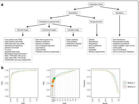
Evaluation criteria: key quantitative performance metrics

Evaluation of methods will rely on one or more

quanti-tative performance metrics (Fig. 2a). The choice of

metric depends on the type of method and data. For ex-ample, for classification tasks with a ground truth, met-rics include the true positive rate (TPR; sensitivity or recall), false positive rate (FPR; 1–specificity), and false discovery rate (FDR). For clustering tasks, common

metrics include the F1 score, adjusted Rand index, nor-malized mutual information, precision, and recall; some of these can be calculated at the cluster level as well as averaged (and optionally weighted) across clusters (e.g., these metrics were used to evaluate clustering methods in our own work [28, 31] and by others [33, 45, 75]). Several of these metrics can also be compared visually to capture the tradeoff between sensitivity and specificity, e.g., using receiver operating characteristic (ROC) curves (TPR versus FPR), TPR versus FDR curves, or preci-sion–recall (PR) curves (Fig. 2b). For imbalanced data-sets, PR curves have been shown to be more informative than ROC curves [76, 77]. These visual metrics can also be summarized as a single number, such as area under the ROC or PR curve; examples from our work include [22, 29]. In addition to the tradeoff between sensitivity and specificity, a method’s‘operating point’is important; in particular, whether the threshold used (e.g., 5% FDR) is calibrated to achieve the specified error rate. We often overlay this onto TPR–FDR curves by filled or open cir-cles (e.g., Fig. 2b, generated using the iCOBRA package [56]); examples from our work include [22,23,25,78].

For methods with continuous-valued output (e.g., ef-fect sizes or abundance estimates), metrics include the root mean square error, distance measures, Pearson cor-relation, sum of absolute log-ratios, log-modulus, and cross-entropy. As above, the choice of metric depends on the type of method and data (e.g., [41, 79] used cor-relation, while [48] used root mean square deviation). Further classes of methods include those generating graphs, phylogenetic trees, overlapping clusters, or dis-tributions; these require more complex metrics. In some cases, custom metrics may need to be developed (e.g., we defined new metrics for topologies of developmental trajectories in [27]). When designing custom metrics, it is important to assess their reliability across a range of prediction values (e.g., [80, 81]). For some metrics, it may also be useful to assess uncertainty, e.g., via confi-dence intervals. In the context of supervised learning, classification or prediction accuracy can be evaluated by cross-validation, bootstrapping, or on a separate test dataset (e.g., [13, 46]). In this case, procedures to split data into training and test sets should be appropriate for the data structure and the prediction task at hand (e.g., leaving out whole samples or chromosomes [82]).

Additional metrics that do not rely on a ground truth include measures of stability, stochasticity, and robust-ness. These measures may be quantified by running methods multiple times using different inputs or sub-sampled data (e.g., we observed substantial variability in

performance for some methods in [29, 31]). ‘Missing

memory requirements (e.g., [27, 29, 31]). Fallback solu-tions such as imputation may be considered in this case [83], although these should be transparently reported. For non-deterministic methods (e.g., with random starts or stochastic optimization), variability in performance when using different random seeds or subsampled data should be characterized. Null comparisons can be con-structed by randomizing group labels such that datasets do not contain any true signal, which can provide infor-mation on error rates (e.g., [22,25,26]). However, these must be designed carefully to avoid confounding by batch or population structure, and to avoid strong within-group batch effects that are not accounted for.

For most benchmarks, multiple metrics will be rele-vant. Focusing on a single metric can give an incomplete view: methods may not be directly comparable if they are designed for different tasks, and different users may

be interested in different aspects of performance. There-fore, a crucial design decision is whether to focus on an overall ranking, e.g., by combining or weighting multiple metrics. In general, it is unlikely that a single method will perform best across all metrics, and performance differences between top-ranked methods for individual metrics can be small. Therefore, a good strategy is to use rankings from multiple metrics to identify a set of con-sistently high-performing methods, and then highlight the different strengths of these methods. For example, in

[31], we identified methods that gave good clustering

performance, and then highlighted differences in run-times among these. In several studies, we have presented results in the form of a graphical summary of perform-ance according to multiple criteria (examples include Fig. 3 in [27] and Fig. 5 in [29] from our work; and Fig.

2 in [39] and Fig. 6 in [32] from other authors).

Evaluation criteria

Comparison to ground truth Discrete target

Quantitative Qualitative

No ground truth Continuous target Complex target

0.00 0.25 0.50 0.75 1.00

0.00 0.25 0.50 0.75 1.00

FPR

TPR TPR

0.01 0.05 0.10.1 0.2 0.3 0.4 0.5 0.6 0.7 0.8 0.9

1

0.00 0.25 0.50 0.75 1.00

FDR

0.00 0.25 0.50 0.75 1.00

0.00 0.25 0.50 0.75 1.00

Recall

Precision

Method_1 Method_2 True positive rate (TPR)

False positive rate (FPR) False discovery rate (FDR) Sensitivity and specificity precision and recall F1 score Adjusted Rand index Normalized mutual information ROC / TPR-FDR / PR curves Area under ROC / PR curves Classification accuracy (supervised)

Root mean square error Distance measures Pearson correlation Sum of absolute log-ratios Log-modulus Cross-entropy

Prediction accuracy (supervised)

Graph similarity Tree similarity Distribution similarity Custom metrics

Stability Stochasticity Robustness Null comparisons Runtime Scalability Memory requirements

User-friendliness Documentation quality Installation procedures Freely available / open source Code quality

Use of unit testing Use of continuous integration

a

b

Fig. 2Summary and examples of performance metrics.aSchematic overview of classes of frequently used performance metrics, including examples (boxes outlined in gray).bExamples of popular visualizations of quantitative performance metrics for classification methods, using reference datasets

with a ground truth. ROC curves (left). TPR versus FDR curves (center);circlesrepresent observed TPR and FDR at typical FDR thresholds of 1, 5, and 10%,

withfilled circlesindicating observed FDR lower than or equal to the imposed threshold. PR curves (right). Visualizations inbwere generated using

iCOBRA R/Bioconductor package [56].FDRfalse discovery rate,FPRfalse positive rate,PRprecision–recall,ROCreceiver operating characteristic,TPRtrue

Identifying methods that consistently underperform can also be useful, to allow readers to avoid these.

Evaluation criteria: secondary measures

In addition to the key quantitative performance met-rics, methods should also be evaluated according to secondary measures, including runtime, scalability, and other computational requirements, as well as qualitative aspects such as user-friendliness, installa-tion procedures, code quality, and documentainstalla-tion quality (Fig. 2a). From the user perspective, the final choice of method may involve tradeoffs according to these measures: an adequately performing method may be preferable to a top-performing method that is especially difficult to use.

In our experience, runtimes and scalability can vary enormously between methods (e.g., in our work, run-times for cytometry clustering algorithms [31] and meta-genome analysis tools [79] ranged across multiple orders of magnitude for the same datasets). Similarly, memory and other computational requirements can vary widely. Runtimes and scalability may be investigated systematic-ally, e.g., by varying the number of cells or genes in a

single-cell RNA-sequencing dataset [28, 29]. In many

cases, there is a tradeoff between performance and com-putational requirements. In practice, if comcom-putational requirements for a top-performing method are prohibi-tive, then a different method may be preferred by some users.

User-friendliness, installation procedures, and docu-mentation quality can also be highly variable [84, 85]. Streamlined installation procedures can be ensured by distributing the method via standard package repositor-ies, such as CRAN and Bioconductor for R, or PyPI for Python. Alternative options include GitHub and other code repositories or institutional websites; however, these options do not provide users with the same guar-antees regarding reliability and documentation quality. Availability across multiple operating systems and within popular programming languages for data analysis is also important. Availability of graphical user interfaces can further extend accessibility, although graphical-only methods hinder reproducibility and are thus difficult to include in a systematic benchmark.

For many users, freely available and open source soft-ware will be preferred, since it is more broadly accessible and can be adapted by experienced users. From the developer perspective, code quality and use of software development best practices, such as unit testing and continuous integration, are also important. Similarly, ad-herence to commonly used data formats (e.g., GFF/GTF files for genomic features, BAM/SAM files for sequence alignment data, or FCS files for flow or mass cytometry data) greatly improves accessibility and extensibility.

High-quality documentation is critical, including help pages and tutorials. Ideally, all code examples in the documentation should be continually tested, e.g., as Bio-conductor does, or through continuous integration.

Interpretation, guidelines, and recommendations

For a truly excellent benchmark, results must be clearly interpreted from the perspective of the intended audi-ence. For method users, results should be summarized in the form of recommendations. An overall ranking of methods (or separate rankings for multiple evaluation criteria) can provide a useful overview. However, as mentioned above, some methods may not be directly comparable (e.g. since they are designed for different tasks), and different users may be interested in different aspects of performance. In addition, it is unlikely that there will be a clear ‘winner’across all criteria, and per-formance differences between top-ranked methods can be small. Therefore, an informative strategy is to use the rankings to identify a set of high-performing methods, and to highlight the different strengths and tradeoffs among these methods. The interpretation may also in-volve biological or other domain knowledge to establish the scientific relevance of differences in performance. Importantly, neutrality principles should be preserved during the interpretation.

For method developers, the conclusions may include guidelines for possible future development of methods. By assisting method developers to focus their research efforts, high-quality benchmarks can have significant im-pact on the progress of methodological research.

Limitations of the benchmark should be transparently discussed. For example, in [27] we used default parame-ters for all methods, while in [31] our datasets relied on manually gated reference cell populations as the ground truth. Without a thorough discussion of limitations, a benchmark runs the risk of misleading readers; in ex-treme cases, this may even harm the broader research field by guiding research efforts in the wrong directions.

Publication and reporting of results

The publication and reporting strategy should emphasize clarity and accessibility. Visualizations summarizing multiple performance metrics can be highly informative

for method users (examples include Fig. 3 in [27] and

Fig. 5 in [29] from our own work; as well as Fig. 6 in [32]). Summary tables are also useful as a reference (e.g., [31, 45]). Additional visualizations, such as flow charts to guide the choice of method for different analyses, are a helpful way to engage the reader (e.g., Fig. 5 in [27]).

For extensive benchmarks, online resources enable readers to interactively explore the results (examples from our work include [27,29], which allow users to

of an interactive website from one of our benchmarks [27], which facilitates exploration of results and assists users with choosing a suitable method. While tradeoffs should be considered in terms of the amount of work re-quired, these efforts are likely to have significant benefit for the community.

In most cases, results will be published in a peer-reviewed article. For a neutral benchmark, the mark will be the main focus of the paper. For a bench-mark to introduce a new method, the results will form one part of the exposition. We highly recommend pub-lishing a preprint prior to peer review (e.g., on bioRxiv or arXiv) to speed up distribution of results, broaden ac-cessibility, and solicit additional feedback. In particular, direct consultation with method authors can generate highly useful feedback (examples from our work are de-scribed in the acknowledgments in [79, 86]). Finally, at publication time, considering open access options will further broaden accessibility.

Enabling future extensions

Since new methods are continually emerging [1], bench-marks can quickly become out of date. To avoid this, a truly excellent benchmark should be extensible. For ex-ample, creating public repositories containing code and data allows other researchers to build on the results to in-clude new methods or datasets, or to try different param-eter settings or pre-processing procedures (examples from our work include [27–31]). In addition to raw data and code, it is useful to distribute pre-processed and/or results data (examples include [28, 29, 56] from our work and [75, 87, 88] from others), especially for computationally intensive benchmarks. This may be combined with an interactive website, where users can upload results from a new method, to be included in an updated comparison

either automatically or by the original authors (e.g., [35,

89, 90]). ‘Continuous’ benchmarks, which are continually updated, are especially convenient (e.g., [91]), but may re-quire significant additional effort.

Reproducible research best practices

Reproducibility of research findings has become an

in-creasing concern in numerous areas of study [92]. In

computational sciences, reproducibility of code and data

analyses has been recognized as a useful ‘minimum

standard’ that enables other researchers to verify

ana-lyses [93]. Access to code and data has previously

enabled method developers to uncover potential errors in published benchmarks due to suboptimal usage of methods [74, 94, 95]. Journal publication policies can play a crucial role in encouraging authors to follow these

practices [96]; experience shows that statements that

code and data are‘available on request’are often

insuffi-cient [97]. In the context of benchmarking, code and

data availability also provides further benefits: for method users, code repositories serve as a source of annotated code to run methods and build analysis pipe-lines, while for developers, code repositories can act as a prototype for future method development work.

Parameter values (including random seeds) and soft-ware versions should be clearly reported to ensure complete reproducibility. For methods that are run using scripts, these will be recorded within the scripts. In R,

the command ‘sessionInfo()’gives a complete summary

of package versions, the version of R, and the operating system. For methods only available via graphical inter-faces, parameters and versions must be recorded manu-ally. Reproducible workflow frameworks, such as the

Galaxy platform [98], can also be helpful. A summary

table or spreadsheet of parameter values and software 2GB

100MB Topology

dynguidelines Tutorial Citation

“

?

Show code </>

Lenses Default Summary (Fig. 2) Method Scalability Stability Usability Accuracy Overall Everything Show/hide columns

Benchmark study Evaluating methods with dynbenchmark Part of

Options Infer trajectories with dyno

Yes I don’t know No

Do you expect multiple disconnected trajectories in the data?

Scalability

1000

COMPUTED

Number of cells

Time limit 1000

10s

10s20s30s40s50s1m10m 20m 30m 40m 50m1h 4h 8h16h 1d 3d

∞

∞

Number of features (genes)

Name

Slingshot

SCORPIUS

Angle

PAGA

Embeddr

MST

Waterfall

TSCAN

Component 1

SLICE

Monocle DDRTree

EIPiGraph linear

100

96

92

89

89

89

89

88

87

83

82

81

942MB

507MB

308MB

559MB Unstable

591MB

572MB

369MB

476MB

516MB

713MB

647MB

573MB 8s

3s

1s

15s

5s

4s

5s

5s

1s

16s

41s

1m

Priors Errors Overall Stability

1h

Memory limit

100MB 500MB 900MB 1GB 3GB 5GB 7GB 9GB 10GB 30GB 50GB 70GB 90GB

∞

∞

Method Accuracy Scalability Stability

!

Unstable

!

Unstable

!

Unstable

!

dynverse

versions can be published as supplementary information along with the publication describing the benchmark (e.g., Supporting Information Table S1 in our study [31]).

Automated workflow management tools and special-ized tools for organizing benchmarks provide sophisti-cated options for setting up benchmarks and creating a reproducible record, including software environments, package versions, and parameter values. Examples

in-clude SummarizedBenchmark [99], DataPackageR [100],

workflowr [101], and Dynamic Statistical Comparisons

[102]. Some tools (e.g., workflowr) also provide stream-lined options for publishing results online. In machine learning, OpenML provides a platform to organize and

share benchmarks [103]. More general tools for

man-aging computational workflows, including Snakemake [104], Make, Bioconda [105], and conda, can be custom-ized to capture setup information. Containerization tools such as Docker and Singularity may be used to encapsu-late a software environment for each method, preserving the package version as well as dependency packages and the operating system, and facilitating distribution of methods to end users (e.g., in our study [27]). Best prac-tices from software development are also useful, includ-ing unit testinclud-ing and continuous integration.

Many free online resources are available for sharing code and data, including GitHub and Bitbucket, reposi-tories for specific data types (e.g., ArrayExpress [106],

the Gene Expression Omnibus [107], and

FlowReposi-tory [108]), and more general data repositories (e.g., fig-share, Dryad, Zenodo, Bioconductor ExperimentHub, and Mendeley Data). Customized resources (examples

from our work include [29, 56]) can be designed when

additional flexibility is needed. Several repositories allow the creation of ‘digital object identifiers’(DOIs) for code or data objects. In general, preference should be given to publicly funded repositories, which provide greater guar-antees for long-term archival stability [84,85].

An extensive literature exists on best practices for

re-producible computational research (e.g., [109]). Some

practices (e.g., containerization) may involve significant additional work; however, in our experience, almost all efforts in this area prove useful, especially by facilitating later extensions by ourselves or other researchers.

Discussion

In this review, we have described a set of key principles for designing a high-quality computational benchmark. In our view, elements of all of these principles are essen-tial. However, we have also emphasized that any bench-mark will involve tradeoffs, due to limited expertise and resources, and that some principles are less central to

the evaluation. Table1provides a summary of examples

of key tradeoffs and pitfalls related to benchmarking,

along with our judgment of how truly ‘essential’ each

principle is.

A number of potential pitfalls may arise from bench-marking studies (Table 1). For example, subjectivity in the choice of datasets or evaluation metrics could bias the results. In particular, a benchmark that relies on un-representative data or metrics that do not translate to real-world scenarios may be misleading by showing poor performance for methods that otherwise perform well. This could harm method users, who may select an in-appropriate method for their analyses, as well as method developers, who may be discouraged from pursuing promising methodological approaches. In extreme cases, this could negatively affect the research field by influen-cing the direction of research efforts. A thorough discus-sion of the limitations of a benchmark can help avoid these issues. Over the longer term, critical evaluations of published benchmarks, so-called meta-benchmarks, will also be informative [10,13,14].

Well-designed benchmarking studies provide highly valuable information for users and developers of compu-tational methods, but require careful consideration of a number of important design principles. In this review, we have discussed a series of guidelines for rigorous benchmarking design and implementation, based on our experiences in computational biology. We hope these guidelines will assist computational researchers to design high-quality, informative benchmarks, which will con-tribute to scientific advances through informed selection of methods by users and targeting of research efforts by developers.

Abbreviations

FDR:False discovery rate; FPR: False positive rate; PR: Precision_–recall;

ROC: Receiver operating characteristic; TPR: True positive rate

Acknowledgments

The authors thank members of the Robinson Lab at the University of Zurich and Saeys Lab at Ghent University for valuable feedback.

Authors_’contributions

LMW proposed the project and drafted the manuscript. WS, RC, CS, AH, PPG, ALB, YS, and MDR contributed ideas and references and contributed to drafting of the manuscript. YS and MDR supervised the project. All authors read and approved the final manuscript.

Funding

MDR acknowledges funding support from the UZH URPP Evolution in Action and from the Swiss National Science Foundation (grant numbers 310030_175841 and CRSII5_177208). In addition, this project has been made possible in part

(grant number 2018–182828 to MDR) by the Chan Zuckerberg Initiative DAF, an

advised fund of the Silicon Valley Community Foundation. LMW was supported by a Forschungskredit (Candoc) grant from the University of Zurich (FK-17-100). WS and RC are supported by the Fonds Wetenschappelijk Onderzoek. YS is an

ISAC Marylou Ingram Scholar. ALB was supported by individual grants BO3139/2–

3 and BO3139/4–3 from the German Research Foundation (DFG) and by the

German Federal Ministry of Education and Research under grant number 01IS18036A (MCML).

Competing interests

Author details

1_{Institute of Molecular Life Sciences, University of Zurich, 8057 Zurich,}

Switzerland.2_{SIB Swiss Institute of Bioinformatics, University of Zurich, 8057} Zurich, Switzerland.3Data Mining and Modelling for Biomedicine, VIB Center for Inflammation Research, 9052 Ghent, Belgium.4_{Department of Applied} Mathematics, Computer Science and Statistics, Ghent University, 9000 Ghent, Belgium.5_{Institute of Medical Informatics, Statistics and Epidemiology,} Technical University of Munich, 81675 Munich, Germany.6Department of Biochemistry, University of Otago, Dunedin 9016, New Zealand.7_{Institute for} Medical Information Processing, Biometry and Epidemiology,

Ludwig-Maximilians-University, 81377 Munich, Germany.8_{Present address:} Friedrich Miescher Institute for Biomedical Research and SIB Swiss Institute of Bioinformatics, 4058 Basel, Switzerland.

References

1. Zappia L, Phipson B, Oshlack A. Exploring the single-cell RNA-seq analysis

landscape with the scRNA-tools database. PLoS Comput Biol. 2018;14: e1006245.

2. Boulesteix A-L, Binder H, Abrahamowicz M, Sauerbrei W. On the necessity

and design of studies comparing statistical methods. Biom J. 2018;60:216_–8.

3. Boulesteix A-L, Lauer S, Eugster MJA. A plea for neutral comparison studies

in computational sciences. PLoS One. 2013;8:e61562.

4. Peters B, Brenner SE, Wang E, Slonim D, Kann MG. Putting benchmarks in

their rightful place: the heart of computational biology. PLoS Comput Biol. 2018;14:e1006494.

5. Boulesteix A-L. Ten simple rules for reducing overoptimistic reporting in

methodological computational research. PLoS Comput Biol. 2015;11: e1004191.

6. Zheng S. Benchmarking: contexts and details matter. Genome Biol. 2017;18:129.

7. Mangul S, Martin LS, Hill BL, Lam AK-M, Distler MG, Zelikovsky A, et al.

Systematic benchmarking of omics computational tools. Nat Commun. 2019;10:1393.

8. Norel R, Rice JJ, Stolovitzky G. The self-assessment trap: can we all be better

than average? Mol Syst Biol. 2011;7:537.

9. Aniba MR, Poch O, Thompson JD. Issues in bioinformatics benchmarking:

the case study of multiple sequence alignment. Nucleic Acids Res. 2010;38:

7353–63.

10. Boulesteix A-L, Wilson R, Hapfelmeier A. Towards evidence-based

computational statistics: lessons from clinical research on the role and design of real-data benchmark studies. BMC Med Res Methodol. 2017; 17:138.

11. Boulesteix A-L, Hable R, Lauer S, Eugster MJA. A statistical framework for

hypothesis testing in real data comparison studies. Am Stat. 2015;69:201–12.

12. Morris TP, White IR, Crowther MJ. Using simulation studies to evaluate

statistical methods. Stat Med. 2019;38:2074–102.

13. Gardner PP, Watson RJ, Morgan XC, Draper JL, Finn RD, Morales SE, et al.

Identifying accurate metagenome and amplicon software via a meta-analysis of sequence to taxonomy benchmarking studies. PeerJ. 2019;7: e6160.

14. Gardner PP, Paterson JM, Ashari-Ghomi F, Umu SU, McGimpsey S, Pawlik A.

A meta-analysis of bioinformatics software benchmarks reveals that publication-bias unduly influences software accuracy. bioRxiv. 2017:092205.

15. Evangelou E, Ioannidis JPA. Meta-analysis methods for genome-wide

association studies and beyond. Nat Rev Genet. 2013;14:379–89.

16. Hong F, Breitling R. A comparison of meta-analysis methods for detecting

differentially expressed genes in microarray experiments. Bioinformatics.

2008;24:374–82.

17. Boutros PC, Margolin AA, Stuart JM, Califano A, Stolovitzky G. Toward better

benchmarking: challenge-based methods assessment in cancer genomics. Genome Biol. 2014;15:462.

18. Friedberg I, Wass MN, Mooney SD, Radivojac P. Ten simple rules for a

community computational challenge. PLoS Comput Biol. 2015;11:e1004150.

19. Van Mechelen I, Boulesteix A-L, Dangl R, Dean N, Guyon I, Hennig C, et al.

Benchmarking in cluster analysis: A white paper. arXiv. 2018;1809:10496.

20. Angers-Loustau A, Petrillo M, Bengtsson-Palme J, Berendonk T, Blais B, Chan

K-G, et al. The challenges of designing a benchmark strategy for bioinformatics pipelines in the identification of antimicrobial resistance determinants using next generation sequencing technologies. F1000Res. 2018;7:459.

21. Ioannidis JPA. Meta-research: why research on research matters. PLoS Biol.

2018;16:e2005468.

22. Weber LM, Nowicka M, Soneson C, Robinson MD. Diffcyt: differential

discovery in high-dimensional cytometry via high-resolution clustering. Commun Biol. 2019;2:183.

23. Nowicka M, Robinson MD. DRIMSeq: a Dirichlet-multinomial framework for

multivariate count outcomes in genomics. F1000Res. 2016;5:1356.

24. Levine JH, Simonds EF, Bendall SC, Davis KL, Amir E-AD, Tadmor MD, et al.

Data-driven phenotypic dissection of AML reveals progenitor-like cells that

correlate with prognosis. Cell. 2015;162:184–97.

25. Zhou X, Lindsay H, Robinson MD. Robustly detecting differential expression

in RNA sequencing data using observation weights. Nucleic Acids Res. 2014; 42:e91.

26. Law CW, Chen Y, Shi W, Smyth GK. Voom: precision weights unlock linear

model analysis tools for RNA-seq read counts. Genome Biol. 2014;15:R29.

27. Saelens W, Cannoodt R, Todorov H, Saeys Y. A comparison of single-cell

trajectory inference methods. Nat Biotechnol. 2019;37:547–54.

28. Duò A, Robinson MD, Soneson C. A systematic performance evaluation of

clustering methods for single-cell RNA-seq data. F1000Res. 2018;7:1141.

29. Soneson C, Robinson MD. Bias, robustness and scalability in single-cell

differential expression analysis. Nat Methods. 2018;15:255–61.

30. Saelens W, Cannoodt R, Saeys Y. A comprehensive evaluation of module

detection methods for gene expression data. Nat Commun. 2018;9:1090.

31. Weber LM, Robinson MD. Comparison of clustering methods for

high-dimensional single-cell flow and mass cytometry data. Cytometry Part A.

2016;89A:1084–96.

32. Korthauer K, Kimes PK, Duvallet C, Reyes A, Subramanian A, Teng M, et al. A

practical guide to methods controlling false discovery rates. Genome Biol. 2019;20:118.

33. Freytag S, Tian L, Lönnstedt I, Ng M, Bahlo M. Comparison of clustering

tools in R for medium-sized 10x genomics single-cell RNA-sequencing data. F1000Research. 2018;7:1297.

34. Baruzzo G, Hayer KE, Kim EJ, Di Camillo B, FitzGerald GA, Grant GR.

Simulation-based comprehensive benchmarking of RNA-seq aligners. Nat

Methods. 2017;14:135–9.

35. Kanitz A, Gypas F, Gruber AJ, Gruber AR, Martin G, Zavolan M. Comparative

assessment of methods for the computational inference of transcript isoform abundance from RNA-seq data. Genome Biol. 2015;16:150.

36. Soneson C, Delorenzi M. A comparison of methods for differential

expression analysis of RNA-seq data. BMC Bioinformatics. 2013;14:91.

37. Rapaport F, Khanin R, Liang Y, Pirun M, Krek A, Zumbo P, et al.

Comprehensive evaluation of differential gene expression analysis methods for RNA-seq data. Genome Biol. 2013;14:R95.

38. Dillies M-A, Rau A, Aubert J, Hennequet-Antier C, Jeanmougin M, Servant N,

et al. A comprehensive evaluation of normalization methods for Illumina

high-throughput RNA sequencing data analysis. Brief Bioinform. 2012;14:671–83.

39. Sage D, Kirshner H, Pengo T, Stuurman N, Min J, Manley S, et al.

Quantitative evaluation of software packages for single-molecule

localization microscopy. Nat Methods. 2015;12:717_–24.

40. Weirauch MT, Cote A, Norel R, Annala M, Zhao Y, Riley TR, et al. Evaluation

of methods for modeling transcription factor sequence specificity. Nat

Biotechnol. 2013;31:126_–34.

41. Costello JC, Heiser LM, Georgii E, Gönen M, Menden MP, Wang NJ, et al. A

community effort to assess and improve drug sensitivity prediction

algorithms. Nat Biotechnol. 2014;32:1202_–12.

42. Küffner R, Zach N, Norel R, Hawe J, Schoenfeld D, Wang L, et al.

Crowdsourced analysis of clinical trial data to predict amyotrophic lateral

sclerosis progression. Nat Biotechnol. 2015;33:51–7.

43. Ewing AD, Houlahan KE, Hu Y, Ellrott K, Caloian C, Yamaguchi TN, et al.

Combining tumor genome simulation with crowdsourcing to benchmark

somatic single-nucleotide-variant detection. Nat Methods. 2015;12:623–30.

44. Hill SM, Heiser LM, Cokelaer T, Unger M, Nesser NK, Carlin DE, et al. Inferring

causal molecular networks: empirical assessment through a

community-based effort. Nat Methods. 2016;13:310–8.

45. Aghaeepour N, Finak G. The FlowCAP Consortium, the DREAM Consortium,

Hoos H, Mosmann TR, et al. critical assessment of automated flow

cytometry data analysis techniques. Nat Methods. 2013;10:228–38.

46. Aghaeepour N, Chattopadhyay P, Chikina M, Dhaene T, Van Gassen S,

Kursa M, et al. A benchmark for evaluation of algorithms for identification of cellular correlates of clinical outcomes. Cytometry Part

47. Moult J, Fidelis K, Kryshtafovych A, Schwede T, Tramontano A. Critical

assessment of methods of protein structure prediction (CASP)_—round XII.

Proteins. 2018;86:7–15.

48. Moult J, Fidelis K, Kryshtafovych A, Schwede T, Tramontano A. Critical

assessment of methods of protein structure prediction: Progress and new

directions in round XI. Proteins. 2016;84:4–14.

49. Sczyrba A, Hofmann P, Belmann P, Koslicki D, Janssen S, Dröge J, et al.

Critical assessment of metagenome interpretation_—a benchmark of

metagenomics software. Nat Methods. 2017;14:1063–71.

50. Earl D, Bradnam K, St John J, Darling A, Lin D, Fass J, et al. Assemblathon 1:

a competitive assessment of de novo short read assembly methods.

Genome Res. 2011;21:2224–41.

51. Bradnam KR, Fass JN, Alexandrov A, Baranay P, Bechner M, Birol I, et al.

Assemblathon 2: evaluating de novo methods of genome assembly in

three vertebrate species. GigaScience. 2013;2:1_–31.

52. Consortium MAQC. The MicroArray quality control (MAQC) project shows

inter- and intraplatform reproducibility of gene expression measurements.

Nature Biotechnol. 2006;24:1151_–61.

53. Consortium MAQC. The microarray quality control (MAQC)-II study of

common practices for the development and validation of microarray-based

predictive models. Nature Biotechnol. 2010;28:827–38.

54. SEQC/MAQC-III Consortium. A comprehensive assessment of RNA-seq

accuracy, reproducibility and information content by the sequencing quality

control Consortium. Nat Biotechnol. 2014;32:903–14.

55. Krusche P, Trigg L, Boutros PC, Mason CE, De La Vega FM, Moore BL, et al.

Best practices for benchmarking germline small-variant calls in human

genomes. Nature Biotechnol. 2019;37:555–60.

56. Soneson C, Robinson MD. iCOBRA: open, reproducible, standardized and

live method benchmarking. Nat Methods. 2016;13:283.

57. Soneson C, Robinson MD. Towards unified quality verification of synthetic

count data with countsimQC. Bioinformatics. 2017;34:691–2.

58. Korthauer K, Chakraborty S, Benjamini Y, Irizarry RA. Detection and accurate

false discovery rate control of differentially methylated regions from whole

genome bisulfite sequencing. Biostatistics. 2018:1_–17.

59. Caboche S, Audebert C, Lemoine Y, Hot D. Comparison of mapping

algorithms used in high-throughput sequencing: application to ion torrent data. BMC Genomics. 2014;15:264.

60. Grimm DG, Azencott C-A, Aicheler F, Gieraths U, MacArthur DG,

Samocha KE, et al. The evaluation of tools used to predict the impact of missense variants is hindered by two types of circularity. Hum Mutat.

2015;36:513–23.

61. Jelizarow M, Guillemot V, Tenenhaus A, Strimmer K, Boulesteix A-L.

Over-optimism in bioinformatics: an illustration. Bioinformatics. 2010;26:

1990–8.

62. Jiang L, Schlesinger F, Davis CA, Zhang Y, Li R, Salit M, et al. Synthetic

spike-in standards for RNA-seq experiments. Genome Res. 2011;21:1543–51.

63. Garalde DR, Snell EA, Jachimowicz D, Sipos B, Lloyd JH, Bruce M, et al.

Highly parallel direct RNA sequencing on an array of nanopores. Nat

Methods. 2018;15:201–6.

64. Fang F, Hodges E, Molaro A, Dean M, Hannon GJ, Smith AD. Genomic

landscape of human allele-specific DNA methylation. Proc Natl Acad Sci U S

A. 2012;109:7332–7.

65. The Tabula Muris Consortium. Single-cell transcriptomics of 20 mouse

organs creates a tabula Muris. Nature. 2018;562:367–72.

66. Zheng GXY, Terry JM, Belgrader P, Ryvkin P, Bent ZW, Wilson R, et al.

Massively parallel digital transcriptional profiling of single cells. Nat Commun. 2017;8:14049.

67. Tian L, Dong X, Freytag S, Lê Cao K-A, Su S, JalalAbadi A, et al.

Benchmarking single cell RNA-sequencing analysis pipelines using mixture

control experiments. Nat Methods. 2019;16:479–87.

68. Arvaniti E, Claassen M. Sensitive detection of rare disease-associated cell

subsets via representation learning. Nat Commun. 2017;8:1–10.

69. Rigaill G, Balzergue S, Brunaud V, Blondet E, Rau A, Rogier O, et al. Synthetic

data sets for the identification of key ingredients for RNA-seq differential

analysis. Brief Bioinform. 2018;19:65–76.

70. Löwes B, Chauve C, Ponty Y, Giegerich R. The BRaliBase dent—a tale of

benchmark design and interpretation. Brief Bioinform. 2017;18:306_–11.

71. Couronné R, Probst P, Boulesteix A-L. Random forest versus logistic regression:

a large-scale benchmark experiment. BMC Bioinform. 2018;19:270.

72. Schneider J, Hapfelmeier A, Thöres S, Obermeier A, Schulz C, Pförringer D,

et al. Mortality risk for acute cholangitis (MAC): a risk prediction model for

in-hospital mortality in patients with acute cholangitis. BMC Gastroenterol. 2016;16:15.

73. Hu Q, Greene CS. Parameter tuning is a key part of dimensionality reduction

via deep variational autoencoders for single cell RNA transcriptomics. Pac

Symp Biocomput. 2019;24:362_–73.

74. Vaquero-Garcia J, Norton S, Barash Y. LeafCutter vs. MAJIQ and comparing

software in the fast moving field of genomics. bioRxiv. 2018:463927.

75. Wiwie C, Baumbach J, Röttger R. Comparing the performance of biomedical

clustering methods. Nat Methods. 2015;12:1033–8.

76. Saito T, Rehmsmeier M. The precision-recall plot is more informative than

the ROC plot when evaluating binary classifiers on imbalanced datasets. PLoS One. 2015;10:e0118432.

77. Powers DMW. Visualization of tradeoff in evaluation: from precision-recall &

PN to LIFT, ROC & BIRD. arXiv. 2015;1505:00401.

78. Soneson C, Love MI, Robinson MD. Differential analyses for RNA-seq:

transcript-level estimates improve gene-transcript-level inferences. F1000Res. 2016;4:1521.

79. Lindgreen S, Adair KL, Gardner PP. An evaluation of the accuracy and speed

of metagenome analysis tools. Sci Rep. 2016;6:19233.

80. Gurevich A, Saveliev V, Vyahhi N, Tesler G. QUAST: quality assessment tool

for genome assemblies. Bioinformatics. 2013;29:1072–5.

81. Narzisi G, Mishra B. Comparing de novo genome assembly: the long and

short of it. PLoS One. 2011;6:e19175.

82. Schreiber J, Singh R, Bilmes J, Noble WS. A pitfall for machine learning

methods aiming to predict across cell types. bioRxiv. 2019:512434.

83. Bischl B, Schiffner J, Weihs C. Benchmarking local classification methods.

Comput Stat. 2013;28:2599–619.

84. Mangul S, Martin LS, Eskin E, Blekhman R. Improving the usability and

archival stability of bioinformatics software. Genome Biol. 2019;20:47.

85. Mangul S, Mosqueiro T, Abdill RJ, Duong D, Mitchell K, Sarwal V, et al.

Challenges and recommendations to improve installability and archival stability of omics computational tools. bioRxiv. 2019:452532.

86. Freyhult EK, Bollback JP, Gardner PP. Exploring genomic dark matter: a

critical assessment of the performance of homology search methods on

noncoding RNA. Genome Res. 2007;17:117–25.

87. Bokulich NA, Rideout JR, Mercurio WG, Shiffer A, Wolfe B, Maurice CF, et al.

Mockrobiota: a public resource for microbiome bioinformatics

benchmarking. mSystems. 2016;1:e00062–16.

88. Conchúir SO, Barlow KA, Pache RA, Ollikainen N, Kundert K, O’Meara MJ,

et al. A web resource for standardized benchmark datasets, metrics, and Rosetta protocols for macromolecular modeling and design. PLoS One. 2015;10:e0130433.

89. Cope LM, Irizarry RA, Jaffee HA, Wu Z, Speed TP. A benchmark for

Affymetrix GeneChip expression measures. Bioinformatics. 2004;20:323_–31.

90. Irizarry RA, Wu Z, Jaffee HA. Comparison of Affymetrix GeneChip expression

measures. Bioinformatics. 2006;22:789–94.

91. Barton M. nucleotid.es: an assembler catalogue.http://nucleotid.es/.

Accessed 4 June 2019.

92. Ioannidis JPA. Why most published research findings are false. PLoS Med.

2005;2:e124.

93. Peng RD. Reproducible research in computational science. Science. 2011;

334:1226–7.

94. Zhou X, Robinson MD. Do count-based differential expression methods

perform poorly when genes are expressed in only one condition? Genome Biol. 2015;16:222.

95. Zhou X, Oshlack A, Robinson MD. miRNA-Seq normalization comparisons

need improvement. RNA. 2013;19:733–4.

96. Hofner B, Schmid M, Edler L. Reproducible research in statistics: a review

and guidelines for the biometrical journal. Biom J. 2016;58:416_–27.

97. Boulesteix A-L, Janitza S, Hornung R, Probst P, Busen H, Hapfelmeier A.

Making complex prediction rules applicable for readers: current practice in

random forest literature and recommendations. Biom J. 2018.https://doi.

org/10.1002/bimj.201700243.

98. Afgan E, Baker D, Batut B, Van Den Beek M, Bouvier D,_Čech M, et al. The

galaxy platform for accessible, reproducible and collaborative biomedical

analyses: 2018 update. Nucleic Acids Res. 2018;46:W537_–44.

99. Kimes PK, Reyes A. Reproducible and replicable comparisons using

SummarizedBenchmark. Bioinformatics. 2019;35:137–9.

101. Blischak J, Carbonetto P, Stephens M. Workflowr: organized + reproducible

+ shareable data science in R.https://jdblischak.github.io/workflowr/.

Accessed 4 June 2019.

102. Wang G, Stephens M, Carbonetto P. DSC: Dynamic Statistical Comparisons

https://stephenslab.github.io/dsc-wiki/index.html. Accessed 4 June 2019. 103. Vanschoren J, van Rijn JN, Bischl B, Torgo L. OpenML: networked science in

machine learning. SIGKDD Explor. 2014;15:49–60.

104. Köster J, Rahmann S. Snakemake—a scalable bioinformatics workflow

engine. Bioinformatics. 2012;28:2520–2.

105. Grüning B, Dale R, Sjödin A, Chapman BA, Rowe J, Tomkins-Tinch CH, et al. Bioconda: sustainable and comprehensive software distribution for the life

sciences. Nat Methods. 2018;15:475–6.

106. Kolesnikov N, Hastings E, Keays M, Melnichuk O, Tang YA, Williams E, et al.

ArrayExpress update_—simplifying data submissions. Nucleic Acids Res.

2015;43:D1113–6.

107. Barrett T, Wilhite SE, Ledoux P, Evangelista C, Kim IF, Tomashevsky M, et al.

NCBI GEO: archive for functional genomics data sets—update. Nucleic

Acids Res. 2013;41:D991_–5.

108. Spidlen J, Breuer K, Rosenberg C, Kotecha N, Brinkman RR. FlowRepository: a resource of annotated flow cytometry datasets associated with

peer-reviewed publications. Cytometry Part A. 2012;81A:727–31.

109. Sandve GK, Nekrutenko A, Taylor J, Hovig E. Ten simple rules for reproducible computational research. PLoS Comput Biol. 2013;9:e1003285.

Publisher’s Note