M E T H O D
Open Access
scAlign: a tool for alignment, integration,
and rare cell identification from scRNA-seq
data
Nelson Johansen
1,2*and Gerald Quon
1,2,3*Abstract
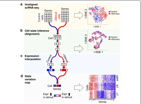
scRNA-seq dataset integration occurs in different contexts, such as the identification of cell type-specific differences in gene expression across conditions or species, or batch effect correction. We present scAlign, an unsupervised deep learning method for data integration that can incorporate partial, overlapping, or a complete set of cell labels, and estimate per-cell differences in gene expression across datasets. scAlign performance is state-of-the-art and robust to cross-dataset variation in cell type-specific expression and cell type composition. We demonstrate that scAlign reveals gene expression programs for rare populations of malaria parasites. Our framework is widely applicable to integration challenges in other domains.
Keywords:scRNA-seq, Data integration, Data harmonization, Alignment, Deep learning, Neural networks, Response to stimulus, Batch effects, Domain adaptation
Background
Single cell RNA sequencing (scRNA-seq) technologies enable the capture of high-resolution snapshots of gene expression activity in individual cells. As the generation of scRNA-seq data accelerates, integrative
analysis of multiple scRNA-seq datasets [1–8] is
be-coming increasingly important. The goal of scRNA-seq data integration is to characterize and eliminate the effect of experimental factors driving expression variation between multiple scRNA-seq datasets, so
that downstream analyses such as clustering [9, 10]
and trajectory inference [10–12] performed on all
datasets jointly are not driven by these factors. Such experimental factors include both technical nuisance
factors such as batch or sequencing protocol [13–18],
as well as biological factors of interest such as in case-control studies [19–22] or speciation [23].
Integrative analyses are challenging due to several factors. First, dataset integration can be viewed as mapping one dataset onto another. For example, in case-control studies for which a pair of scRNA-seq
datasets are generated from biological replicate popu-lations before and after stimulus, functionally matched cell types across datasets must be identified and aligned in order to estimate cell type-specific response to stimulus. The more differential the response of the individual cell types, the more complex a mapping is required. Therefore, integrative tools must be able to freely scale up or down the complexity of their map-ping functions to successfully perform integration de-pending on the heterogeneity of cell type-specific response to stimulus. In the extreme case where some cell types are present in only a subset of conditions being integrated, this poses additional mapping challenges since there may not be a 1-1 correspondence between types across conditions. Second, current integrative tools can be separated into two exclusive sets: those that require all cells from all datasets to have known cell type labels (su-pervised) and those that do not make use of any cell type labels (unsupervised). Consequently, when only a subset of cells can be labeled with high accuracy, or if only one data-set is labeled (as is the case when reference annotated cell atlases are available [23–28]), this partial set of labels cur-rently cannot be used in data integration. Third, measured transcriptomes even for homogeneous populations of cells occupy a continuum of cell states, for both technical [29,
© The Author(s). 2019Open AccessThis article is distributed under the terms of the Creative Commons Attribution 4.0 International License (http://creativecommons.org/licenses/by/4.0/), which permits unrestricted use, distribution, and reproduction in any medium, provided you give appropriate credit to the original author(s) and the source, provide a link to the Creative Commons license, and indicate if changes were made. The Creative Commons Public Domain Dedication waiver (http://creativecommons.org/publicdomain/zero/1.0/) applies to the data made available in this article, unless otherwise stated.
* Correspondence:[email protected];[email protected]
1Graduate Group in Computer Science, University of California, Davis, Davis,
CA, USA
30] and biological [31–33] reasons. Thus, individual cells cannot be matched exactly across datasets. Therefore, downstream analysis of integrated datasets typically involves clustering cells across datasets to find match-ing cell types and estimatmatch-ing cell type-specific differ-ences across datasets. The clustering step makes it difficult to find rare cell populations that differ be-tween datasets.
Here, we present scAlign, a deep learning-based method for scRNA-seq alignment. scAlign performs single cell alignment of scRNA-seq data by learning a bidirectional mapping between cells sequenced within individual datasets, and a low-dimensional alignment space in which cells group by function and type, re-gardless of the dataset in which it was sequenced.
This bidirectional map enables users to generate a representation of what the same cell looks like under each individual dataset and therefore simulate a matched experiment in which the exact same cell is sequenced simultaneously under different conditions. Compared to previous approaches, scAlign can scale in alignment power due to its neural network design, and it can optionally use partial, overlapping, or a complete set of cell type labels in one or more of the input datasets. We demonstrate that scAlign outper-forms existing alignment methods including Seurat [3, 34], scVI [7], MNN [2], scanorama [8], scmap [5], MINT [1], and scMerge [4], particularly when individ-ual cell types exhibit strong dataset-specific signatures such as heterogeneous responses to stimulus. While Cell state inference
(Alignment)
State variation map Unaligned scRNA-seq
+Stimuli cells Genes
Control cells
Genes Genes
t-SNE 2
t-SNE 1
t-SNE 1 Expression
interpolation
Genes
Cell
Cell
Expr in stimuli
Expr in stimuli
t-SNE 2
Genes
Cells
a
b
c
d
Control +Stimulus
Control +Stimulus
MPP
ST
LT
[image:2.595.58.540.87.442.2]misalignment of cell types unique to one dataset is an inherent challenge for any alignment technique, we show that scAlign produces minimal false positive matchings. Furthermore, we show that our bidirec-tional map enables identification of changes in rare cell types that cannot be identified from alignment and data analysis steps performed in isolation. We also demonstrate the utility of scAlign in identifying changes in expression associated with sexual commit-ment in malaria parasites and posit that scAlign may be used to perform alignment in domains other than single cell genomics as well.
Results
[image:3.595.62.539.86.475.2]component of scAlign is the construction of an align-ment space using scRNA-seq data from all conditions, in which cells of the same functional type are indis-tinguishable, regardless of which condition they were sequenced in (Fig.1(b)). This alignment space represents an unsupervised dimensionality reduction of scRNA-seq data from genome-wide expression measurements to a low-dimensional manifold, using a shared deep encoder neural network trained across all conditions. Unlike autoencoders, which share a similar architecture to scA-lign but use a different objective function, our low-dimensional manifold is learned by training the neural network to simultaneously encourage overlap of cells in the state space from across conditions (thus performing alignment), yet also preserving the pairwise cell-cell simi-larity within each condition (and therefore minimizing distortion of gene expression). Optionally, scAlign can take as input a partial or full set of cell annotations in one or more conditions, which will encourage the alignment to cluster cells of the same type in alignment space.
In the second component of scAlign (Fig. 1 (c)),
we train condition-specific deep decoder networks capable of projecting individual cells from the align-ment space back to the gene expression space of each input condition, regardless of what condition the cell is originally sequenced in. We use these de-coders to measure per-cell and per-gene variation of expression across conditions, which we term the cell state variation map. In the case of integrating two conditions, this cell state variation map estimates a paired difference in expression of the same cell
across conditions (Fig. 1 (d)). scAlign therefore seeks
to re-create the ideal experiment in which the exact same cell is sequenced before and after a stimulus in a case-control study, for example.
scAlign captures cell type-specific response to stimulus
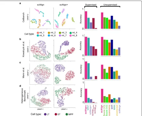
We first benchmarked the alignment component of scA-lign using data from four publicly available scRNA-seq studies for which the same cell populations were Fig. 3Joint analysis of cells from all conditions leads to more accurate clustering of cell types compared to independent analysis of individual conditions.
[image:4.595.60.539.87.412.2]sequenced under different conditions and for which the
cell type labels were obtained experimentally (Fig. 2,
Additional file1: Figure S1). Our first benchmark is Cell-Bench [35], a dataset consisting of three human lung adenocarcinoma cell lines (HCC827, H1975, H2228) that were sequenced using three different protocols (CEL-Seq2, 10x Chromium, Drop-Seq Dolomite) as well as at varying relative concentrations of either RNA content or numbers of cells in a mixture. While the alignment of the homogeneous cell populations sequenced across protocols was trivial and did not require data integration methods (Additional file1: Figure S2), alignment of RNA mixtures across protocols was more challenging and more clearly il-lustrated the performance advantage of scAlign (Fig.2a). We additionally benchmarked alignment methods using data generated by Kowalczyk et al. [36] and Mann et al. [37] on three hematopoietic cell types (LT-HSC, ST-HSC, MPP) collected from the C57BL/6 mouse
strain at approximately 2 months (“young”) and 2
years (“old”) of age. Mann et al. additionally chal-lenged the mice with an LPS or a control stimulus. Similar to our results with CellBench, scAlign outper-forms other approaches on both of these benchmarks
(Fig. 2b, c). The results of scAlign in these
compari-sons were robust to network depth, width, and input
features (Additional file 1: Figure S3 and Figure S4)
along with choice of hyper parameters.
To better understand why the relative performance of the other methods was inconsistent across benchmarks (Fig. 2a–c), we next characterized the difficulty of each benchmark for alignment. For each cell type in each benchmark, we identified cell type marker genes by computing the differentially expressed genes (DEGs) between cell types, individually for each condition. We observed considerable overlap in the cell type marker
genes (Additional file 1: Figure S5), suggesting these
benchmarks may be less challenging to align and there-fore more difficult to distinguish alignment methods from each other. We therefore constructed a novel benchmark termed HeterogeneousBenchmark by com-bining published scRNA-seq data on hematopoietic cells measured across different studies and stimuli. This benchmark yields smaller overlap in cell type marker genes (Additional file1: Figure S5), which makes it more challenging to align. On HeterogeneousBenchmark, we
find that scAlign’s performance is robustly superior,
while Seurat and Scanorama also outperform the
remaining methods (Fig.2d).
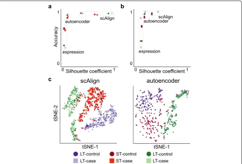
scAlign simultaneously aligns scRNA-seq from multiple conditions and performs a non-linear dimensionality reduction on the transcriptomes. This is advantageous be-cause dimensionality reduction is a first step to a number of downstream tasks, such as clustering into putative cell types [38] and trajectory inference [39–41]. Dimensionality reduction of cell types generally improves when more data is used to compute the embedding dimensions, and so we hypothesized that established cell types will cluster better in scAlign’s embedding space in part due to the fact we are defining a single embedding space using data from multiple conditions. We therefore compared the clustering of known cell types in the scAlign embedding space to an autoencoder neural network that uses the same architecture and number of parameters as scAlign, but is trained on each condition separately (see the
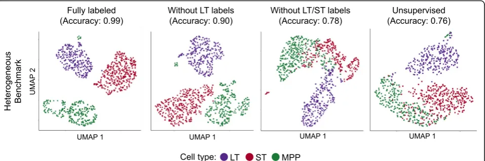
“Methods” section). In two of the three benchmarks we tested, we found that known cell types cluster more closely and are more distinct in scAlign embed-ding space compared to that of the corresponembed-ding autoencoder (Fig. 3, Additional file 1: Figure S6), sug-gesting scAlign’s embedding space benefits from pooling cells from across all conditions. Furthermore, by pooling cells into a common embedding space, scAlign can Fig. 4Semi-supervised alignment mode of scAlign enables use of partial sets of cell type labels. UMAP visualization of the HeterogenousBenchmark after alignment with scAlign+ trained withalabels for all cells in both conditions,bafter removal of labels for LT-HSC HSC in the stimulated condition,
[image:5.595.60.539.88.247.2]identify new subpopulations within known cell type clus-ters (Additional file1: Figure S7).
A unique feature of scAlign is that it can optionally use cell type labels for a subset of (or all) cells if available, but does not require any labels by default. In other words, scAlign can perform unsupervised, semi-supervised, or fully supervised alignment. One example of a use case would be when a labeled, highly-quality cell atlas is avail-able, it can be used to label cells sequenced from a newer, smaller study. Figure2a–d illustrate, for each of the four benchmarks, that scAlign performance improves when cell type labels are available at training time and exceeds the performance of other supervised methods such as MINT [30], scMerge [4], and scmap [5]. Even when only a subset of cells from one condition have labels available for semi-supervised training, scAlign performance improves compared to a strictly unsupervised alignment, though still lower than a fully supervised scAlign+ (Fig.4, Add-itional file 1: Figure S8). When provided with labels, the cell-cell similarity matrix of the supervised scAlign method is qualitatively similar to the cell-cell similarity
matrix of cells in the original gene expression space as well as the unsupervised scAlign alignment space, suggest-ing the inferred alignment space is robust to addsuggest-ing labels during alignment (Additional file1: Figure S9).
scAlign is robust to large differences in cell type representation across conditions
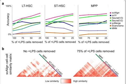
Besides cell type-specific responses to stimuli, we reasoned that the other factor that determines alignment difficulty is the difference in the representation (or proportion present) of each cell type across conditions. For example, cell types unique to one condition may pose challenges to alignment because there are no functionally matched cell types in the other conditions. We therefore explored the behavior of scAlign and other approaches when the rela-tive proportion of cell types varies significantly between the conditions being aligned.
We performed a series of experiments on the Kowalczyk et al. benchmark where we measured alignment per-formance of all methods as we removed an increasing proportion of cells from each cell type from the old
a
b
[image:6.595.57.541.354.676.2]mouse condition (Fig. 5). While scAlign had superior performance across all experiments and was most ro-bust to varying cell type proportions, surprisingly, we found that other methods were generally robust as well. Removing even 75% of the cells of a given type only led to a median drop of 11% in accuracy across the tested methods. When we repeated these experiments on the Mann et al. benchmark, we generally found a larger de-crease in performance as we removed more cells from each type compared to the Kowalczyk et al. benchmark, though scAlign still outperformed all other methods (Additional file1: Figure S10).
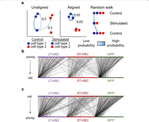
We next investigated the factors that underlie scA-lign’s robustness to imbalanced cell type representation
across conditions. scAlign optimizes an objective
function that minimizes the difference between the pair-wise cell-cell similarity matrix in gene expression space and the pairwise cell-cell similarity matrix implied in the alignment space when performing random walks of length two (Fig. 6a). The random walk starts with a cell sequenced in one condition, then moves to a cell se-quenced in the other condition based on proximity in alignment space. The walk then returns to a different cell (excluding the starting cell) in the original condition, also based on proximity in alignment space. For every cell in each condition, we calculated the frequency that such random walks (initiated from the other condition) pass through it (Fig. 6b, c). We found that a select few representatives for each cell type are visited much more frequently than others and that even when those cells
Fig. 6Random walks during scAlign training frequently visit a small number of hub cells.aSchematic of the cross condition round trip random walk prior to and after training of scAlign.bVisualization of the probability of a walk from each individual young cell (top) to each individual old cell (bottom) after training scAlign on the Kowalczyk et al. benchmark. Edge density represents the magnitude of the probability of a given walk.
[image:7.595.58.538.283.675.2]are removed from the condition, another cell is automat-ically selected as a replacement (Additional file1: Figure S11). This suggests that a given cell type in one con-dition only depends on a few cells of the same type in the other condition to align properly, and so scA-lign ascA-lignment does not need every cell type to be represented in the same proportion across conditions.
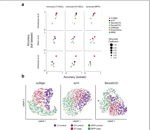
In the above experiments, we have aligned conditions in which the same set of cell types are present in all con-ditions. We next explored the behavior of scAlign and other approaches when there are cell types represented in only a subset of the conditions. We expect such sce-narios to arise when only a subset of cell types respond
to, or are targeted by, a stimulus or condition. For each of our benchmarks, we removed one cell type from one of the conditions (e.g., the LPS condition of the Mann benchmark or the old mouse condition of the Kowalczyk benchmark) and aligned the control and stimulated condi-tions to determine the extent to which the unique popula-tion maintained separapopula-tion from other cell types after alignment. Figure7a demonstrates that in eight out of nine cases, scAlign outperforms other alignment methods in terms of classification accuracy. Even in cases where the alignment accuracy was similar between methods, scAlign visually separates cell types in its alignment space more so than other approaches such as Scanorama and Seurat
a
b
[image:8.595.58.540.267.684.2](Fig. 7b). For other approaches, the separation of different cell types within the same condition shrinks when one cell type is removed (Additional file1: Figure S12).
scAlign interpolates gene expression accurately
One of the more novel features of scAlign is the ability to map each cell from the alignment space back into the gene expression space of each of the original conditions, regardless of which condition the cell was originally sequenced in. This mapping is performed through interpolation: for each condition, we learn a mapping from the alignment space back to gene expression space using cells sequenced in that condition, then apply the map to all cells sequenced in all other conditions. This interpolation procedure enables measurement of vari-ation in gene expression for the same cell state across multiple conditions and simulates the ideal experiment in which the exact same cell is sequenced before and after a stimulus is applied, and the variation in gene ex-pression is subsequently measured.
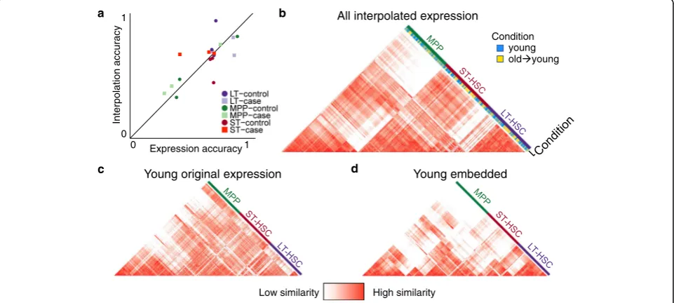
To measure the accuracy of scAlign interpolation, for each of the three hematopoietic benchmarks, we trained de-coder neural networks to map cells from the alignment space back into each of the case and control conditions. We then measured interpolation accuracy as the accuracy of a classifier trained on the original gene expression profiles of
cells sequenced under one condition (e.g., stimulated), when used to classify cells that have been interpolated from the other condition (e.g., control). Comparing this interpolation accuracy to cross-validation accuracy of classifying cells in their original condition using the original measured gene ex-pression profiles, we see that interpolation accuracy is simi-lar to expression accuracy (Fig. 8a), suggesting that cells maintain their general type when mapped into another condition.
Figure8b illustrates the cell-cell similarity matrix com-puted in gene expression space of hematopoietic cells collected in the Kowalczyk study, when including cells sequenced in the young mice, as well as cells that have been interpolated from the old mice into the young condi-tion. We see that cells cluster largely by cell type (LT-HSC, ST-(LT-HSC, MPP) and not by their condition of origin. Furthermore, by computing a state variance map from the interpolation of all cells into both conditions, we identify differentially expressed genes that were not identified by traditional differential expression analysis (Additional file1: Figure S13). This demonstrates that the encoding and interpolation process maintains data fidelity, even though the encoder is trained to align data from multiple condi-tions and is not explicitly trained to minimize
reconstruc-tion error like typical autoencoders. Figure 8c and d
further illustrate that the cell-cell similarity matrix in
Condition young old young
All interpolated expression
Young original expression Young embedded
1 0 Expression accuracy 0
1
y
c
ar
u
c
c
a
n
oit
al
o
pr
et
nI
a b
c d
High similarity Low similarity
0 5 0 5 0
[image:9.595.58.539.419.635.2]embedding space is faithful to the cell-cell similarity matrix in the original gene expression space.
Interpolation identifies early gametocyte markers of the
engineered ap2-g-dd strain ofP. falciparum
We next applied scAlign to identify genes associated with early steps of sexual differentiation inPlasmodium
falcip-arum, the most widespread and virulent human malaria
parasite. Briefly, the clinical symptoms of infection are the result of exponential growth of asexual parasites within red blood cells, while parasite transmission depends on the formation of the non-replicating male and female sexual stages necessary for infection of the parasite’s mos-quito vector. During each round of asexual replication, a
subpopulation of parasites will activate expression of the ap2-g gene, which encodes the transcriptional master regulator of sexual differentiation, to initiate sexual differ-entiation. While the geneap2-gis a known master regula-tor of sexual commitment, and its expression is necessary
for sexual commitment, the events which follow ap2-g
activation and lead to full sexual commitment are un-known [42]. Furthermore,ap2-gexpression is restricted to a minor subset of parasites, making the identification of the precise stage of the life cycle when sexual commitment occurs a challenging task.
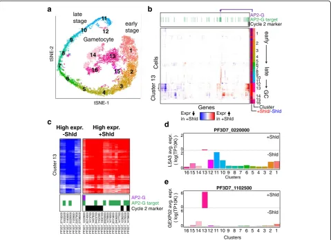
Figure 9a illustrates the alignment space of parasites
which are either capable of ap2-g expression and will
contain an ap2-g-expressing subpopulation in the initial
a
LSA3 avg. expr
.
( log(TP10K) )
PF3D7_0220000
16 15 14 13 12 11 10 9 8 7 6 5 4 3 2 1
PF3D7_1102500
Clusters
16 15 14 13 12 11 10 9 8 7 6 5 4 3 2 1 tSNE-1 tSNE-2 Cluster 13 early GC late Cells
Cycle 2 marker
AP2-G target AP2-G Genes 1 2 3 4 5 6 7 8 9 10 11 12 13 14 15 16
c
3 1 r et s ul C High expr. -Shld High expr. +Shld AP2-G AP2-G targetCycle 2 marker
d
PF3D7_12 2 2 60 0 PF3D7_02 1 4 30 0 PF3D7_14 7 3 70 0 PF3D7_14 6 7 60 0 PF3D7_04 2 3 70 0 P F 3 D 7 _ 1 1 02500 PF3D7_13 0 2 10 0 PF3D7_09 2 0 00 0 PF3D7_14 7 8 90 0 PF3D7_14 7 4 00 0 PF3D7_03 1 5 60 0 PF3D7_04 0 6 20 0 PF3D7_14 7 7 70 0 PF3D7_12 3 6 20 0 P F 3 D 7 _ 1 4765 00 P F 3 D 7 _ 1 4766 00 PF 3 D 7_ 07 1 6 20 0 PF 3D 7_10 0 2 20 0 PF3D 7 _ 1 1 49000 PF 3D 7_02 2 0 00 0 PF3 D 7_ 1 1 20600 PF 3 D 7 _02 0 7 9 0 0 PF 3 D 7 _07 0 8 5 0 0 early stage late stage Gametocyte 1 2 3 4 5 6 8 9 10 11 12 13 14 15 16 7b
Cluster +Shld/-Shld Expr in +Shld Expr in +Shlde
+Shld -Shld +Shld -Shld Clusters GEXP02 avg. expr .( log(TP10K) )
2 0 2 0 6 0 6 0
[image:10.595.59.539.266.613.2]stages of sexual differentiation (+Shld), or areap2-g defi-cient and therefore all committed to continued asexual
growth (−Shld). As was observed in the original paper
[42], the +/−Shld cells fall into clusters that can be or-dered by time points in their life cycle (Fig.9a). scAlign alignment maintains the gametocytes from the +Shld condition as a distinct population that is not aligned to
any parasite population from the −Shld condition,
whereas other tested methods are unable to isolate the gametocyte population (Additional file1: Figure S14).
To further investigate how scAlign is able to maintain the gametocytes as a distinct population after alignment, we looked at the random walks performed by the gam-etocyte cells to see which cells from the−Shld condition they walked to, and found that scAlign maps a very small number of cells from similar surrounding clusters into the peripheral region of alignment space near the
gametocytes. These −Shld cells in the periphery of the
gametocyte cluster allow the gametocytes to use those
cells as “anchors” in their random walk and maintain
their overall separation from the−Shld cells. To confirm
this hypothesis, we removed the contaminating −Shld
parasites used as anchors by the +Shld gametocytes and
re-aligned the +Shld and reduced set of −Shld cells.
After realignment, we found that scAlign “sacrificed”
parasites from similar surrounding clusters to act as new anchors and preserve the distinct +Shld gametocytes as a distinct population (Additional file1: Figure S15).
Because the +Shld and−Shld cells form a set of clusters that we could order from early stage to late stage then gametocytes (+Shld), we hypothesized that the state vari-ation map computed by scAlign could reveal where in the life cycle sexual-committing cells (a subset of +Shld cells) distinguished themselves in variation from asexual-committing cells (all−Shld cells). Using the interpolation component of scAlign, we projected each cell sequenced from each condition in the alignment space into the expression space of both of the +/−Shld conditions. By tak-ing the difference in interpolated expression for each cell
between the +Shld and −Shld transcriptomes, we
com-puted a state variation map illustrating the predicted differ-ence between the two conditions along the entire life cycle (Fig.9b). From the state variation map, we observed few overall predicted differences in gene expression between the two conditions across most stages of the life cycle, ex-cept within a cluster of cells containing the gametocytes specific to the +Shld condition (Fig. 9b, cluster 13). In other words, gametocytes from cluster 13 exhibited the lar-gest predicted differential gene expression between the
+Shld gametocytes and neighboring −Shld
non-gametocyte parasites. We verified that scAlign
interpolation uses cells from neighboring clusters to pre-dict−Shld expression within cluster 13 (Fig.9d, e, see the
“Methods”section).
Over all 661 highly variable genes we analyzed, we found the predicted differentially expressed genes in cluster 13 are enriched in genes previously established to play a role in gametocyte maturation (Fig. 9b) (p= 1.2 × 10⁻⁶, Wilcox
rank sum test), including pfg27 (PF3D7_1302100) and
etramp4(PF3D7_0423700) [44]. Furthermore, for the genes we predict to be upregulated in cluster 13 of the +Shld con-dition, we observed an enrichment ofap2-gtargets identi-fied via ChIP-Seq [43] (p= 6.8 × 10⁻⁷, Wilcox rank sum test). This upregulation of ap2-gtargets is consistent with the fact that cells that have entered the gametocyte stage must have turned onap2-gexpression, but that−Shld cells cannot expressap2-g. Our state variation map identifies an additional eight genes not reported by Bancells and col-leagues as playing a role in gametocyte maturation, but that are predicted to differ between +/−Shld (Fig.9c). Taken in total, these results suggest the other genes we have pre-dicted as differing between +/−Shld may also play a role in gametocyte conversion (Fig.9b, c).
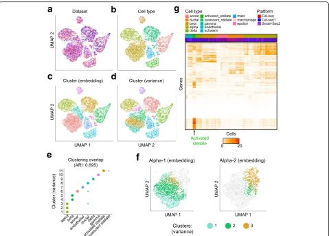
scAlign identifies highly variable genes in pancreatic islet cells sequenced using multiple protocols
We next tested scAlign’s ability to infer an alignment space across more than two conditions by aligning pancreatic islet cells [15] derived from 8 donors and captured using four different protocols (CEL-Seq, CEL-Seq2, Smart-Seq2, and C1). The un-aligned pancreatic islet cells separate by protocol and not cell type, indicating strong protocol-specific effects which are removed after scAlign alignment (Additional file 1: Figure S16 and Figure S17a). scAlign outperforms Seurat and scVI in terms of composite align-ment accuracy on this dataset (Additional file 1: Figure S17b-c). Interestingly, scAlign preserves the stellate, ductal, and gamma cell types as separate clusters of cells, even though these three groups are represented in only a subset of the four protocols.
Having aligned the pancreatic islet cells into an
align-ment space, we next computed scAlign’s state variance
map to identify cell types and genes exhibiting high expression variation across three protocols to provide insight into how the choice of protocol affects gene
ex-pression measurement (Fig. 10a–d). Here, we excluded
cells, and we confirmed these genes to be enriched in
gene functions related to stellate function
(Additional file2).
Robust cell type marker genes drive alignments
To gain insight into the general principles and genes used by scAlign to perform alignment, we performed a series of in silico expression perturbation experiments. scAlign uses the same feed-forward network to reduce the dimensionality of cells from all input conditions. We therefore hypothesized that scAlign is implicitly identify-ing cell type marker genes that are invariant (robust) across conditions and using these marker genes to per-form dimensionality reduction as they will naturally cause similar cell types across conditions to map to the same regions of alignment space. We tested this
[image:12.595.59.539.86.429.2]moving an average of 5.2-fold more than the control sets (Additional file1: Figure S18).
We next sought to evaluate the extent to which
scAlign’s unique random walk-based objective
func-tion contributes to its alignment accuracy. Tradifunc-tional neural networks that focus on unsupervised dimen-sionality reduction such as autoencoders use an ob-jective function that explicitly learn embeddings that minimize the reconstruction loss of each cell. In con-trast, the scAlign objective function simultaneously encourages embeddings to maintain cell-cell similarity within condition, as well as match cells in the align-ment space across conditions. We therefore evaluated the utility of scAlign’s objective function by substitut-ing scAlign’s loss function for a classic reconstruction loss-based autoencoder loss function. This autoenco-der shares the same number of layers and nodes per layer as scAlign and furthermore uses a shared en-coder across all conditions similar to scAlign, but
unique decoders for each condition (see the
“Methods” section). Both the autoencoder and scAlign therefore have the same number of parameters and therefore equal model capacity, and only differ by their respective objective functions. When comparing this autoencoder to scAlign on each of our four benchmarks, we found that the autoencoder was able to achieve similar accuracy on benchmarks with min-imal cell type-specific condition effects, such as
Cell-bench and Kowalczyk et al. (Additional file 1: Figure
S19a-b). However, on more challenging benchmarks such as Mann et al. and our HeterogeneousBench-mark, the autoencoder performed worse than scAlign
(Additional file 1: Figure S19c-d). Furthermore, the
autoencoder did not maintain the cell-cell similarity matrix in embedding space as well as scAlign
(Add-itional file 1: Figure S19 and Figure S20), suggesting
the low-dimensional embeddings learned by the auto-encoder may not as faithfully recapitulate the gene expression inputs.
Discussion
We have shown that scAlign outperforms other integra-tion approaches, particularly when there are strong cell type-specific differences across conditions, or when there is an imbalance in cell type representation across condi-tions. Compared to other approaches, scAlign will be particularly useful in the context where only some cell type labels are available in one or more conditions. We envision two scenarios where this may occur. First, with the increasing number of cell atlases [23–28] that are ac-curately labeled by domain experts and are now publicly available, scAlign can take advantage of the accurate la-beling of these atlases to annotate new datasets that lack labels. Second, marker genes may be available for only a
subset of cell types such as specific hematopoietic cells, in which case only a subset of cells may be reliably la-beled. Even when marker genes are available, markers may not be unique to individual cell types and technical factors such as dropout may prevent truly expressed markers from being detected in the RNA. Here, scAlign can be used in conjunction with only the most confident labeled cells, or can even be used when there is overlap-ping labels (due to marker uncertainty).
Another advantage of scAlign over other integra-tion methods is the improved ability to detect rare differential expression events between conditions. For typical alignment methods, once the effect of condition is removed via alignment, cells must still be clustered into putative cell types in order to iden-tify which cells match across condition, and then perform an unpaired differential expression test within each cluster to identify condition-specific dif-ferences. The need to cluster cells means the detec-tion of rare cell types can be highly sensitive to the choice of clustering algorithm or parameters. In con-trast, through interpolation, scAlign predicts how each individual cell within the alignment space dif-fers in expression between any of the input condi-tions, effectively performing a paired (or matched) differential expression calculation per-cell without the need to cluster. The result is scAlign can detect the presence of rare cell populations that differ in
expression across conditions (Fig. 9).
scAlign implements two approaches to aligning more than two conditions simultaneously. In the reference-based alignment, a single reference condition is established and all other conditions are being aligned against the reference (Additional file1: Figure S21). This is expected to work well when all cell types are represented in all conditions, and has the benefit of speed. Alternatively, the all-pairs align-ment mode performs an all-pairwise set of alignalign-ments sim-ultaneously, which will be more robust to the presence of cell types only represented in a subset of the conditions.
generally, the design of scAlign’s neural network architec-ture and loss functions are general and not specific to scRNA-seq data. We therefore expect that scAlign should be applicable to any problem in which the study design consists of comparing two or more groups of unmatched samples, and where we expect there to be subpopulations of individuals within each group.
Here, we have primarily compared scAlign against un-supervised alignment methods. In our un-supervised alignment results, scAlign compared favorably against the supervised methods MINT [1] and scmap [5] when assuming all cells are labeled. In the context of alignment, however, we rea-soned that if a complete set of labels are available for all cells and conditions, then addressing the task of alignment is less useful, because cells of the same type across condi-tions can be directly compared via per-cell type differential expression analysis without alignment. Alternatively, in those contexts, each matching pair of cell types across con-ditions can be independently aligned using the unsuper-vised scAlign (or other unsuperunsuper-vised methods) to identify matching subpopulations of cells.
The tasks of transcriptional alignment and batch correc-tion of scRNA-seq data are intimately related, as one can view the biological condition of a cell as a batch whose ef-fect should be removed before integrated data analysis. Compared to batch correction methods, scAlign leverages the flexibility of neural networks to perform alignment where cell states might exhibit heterogeneous responses to stimuli, yet through interpolation provides the inter-pretability that canonical batch correction methods enjoy.
Like all other supervised and unsupervised alignment methods, scAlign makes an underlying assumption that the two or more conditions used as input make sense biologic-ally to align. That is, alignment methods assume that there are at least some common cell types between conditions that share some functional origin or similarity, that should be matched across conditions, even if they differ in state (e.g., expression) due to condition or stimulus. To the best of our knowledge, there is no procedure or strategy for identifying datasets that should not be aligned due to lack of matching cell types. As a result, any alignment method when applied to datasets which contain unrelated or dis-similar cell types can potentially lead to false positive matchings. This limitation is not specific to alignment methods; scRNA-seq analysis tools designed for other pur-poses, such as trajectory inference, assume that a trajectory exists in the input data in the first place, and will return a trajectory regardless of whether it makes sense to do so. scRNA-seq tools in general are useful for generating hy-potheses (in the case of alignment, hyhy-potheses about which cell types match across conditions, and how they differ), but need to be used cautiously by downstream users.
A related concern is the performance of alignment methods when there exist condition-specific cell types that
have no matching cell type in another condition. In our experiments, we show that scAlign outperforms other alignment methods in this scenario by choosing a small number of cells from a matching cell type and placing those small numbers of cells in the same region of alignment space as the condition-specific cell type; in other words, scAlign purposefully mis-aligns a small number of cells. scAlign tends to sacri-fice a small number of cells because its objective function minimizes the distortion of the cell-cell pair-wise similarity matrix within each input condition, and so sacrificing many cells would lead to a large distortion of the pairwise similarity matrix.
As a neural network-based method, scAlign usage re-quires specification of the network architecture before training, defined by the number of layers and number of nodes per layer. In our results, we have shown scAlign is largely robust to the size of the architecture, in part be-cause in addition to the ridge penalty we apply to the weights of the network, our objective function minimizes the difference between the similarity matrix in the ori-ginal expression and alignment spaces, which also acts as a form of data-driven regularization.
Methods
Methods overview
The scAlign method consists of two steps: (1) alignment, which learns a mapping from gene expression space of individual conditions into a common alignment space, and (2) interpolation, which learns a mapping from the common alignment space back to the gene expression space of the original conditions.
Pairwise scRNA-seq alignment with scAlign
We define the alignment task as identifying a low-dimensional embedding space (termed the alignment space) in which functionally similar cells map to the same coordinates. Viewed from the lens of perturbation studies, if sequencing a cell immediately before and after stimulus were possible, alignment would bring cells post-stimulus into the same region of alignment space as the cell before stimulus, therefore removing the effect of the stimulus.
scAlign encodes the alignment space by extending the recent approach of learning by association for
neural networks [45, 46] into a unified framework for
both unsupervised and supervised applications. For notational simplicity, we will assume we are aligning scRNA-seq data from a pair of conditions, though the framework extends to multiple conditions (see below). Let !xsi and !xtj be vectors of length G that represent
the gene expression profiles of cells i and j in
condi-tions s and t, respectively. Similarly, let !esi and !etj
space embedding of cells i and j in conditions s and
t, respectively, where the embeddings represent the
linear activations of the final output layer of an en-coder neural network.
scAlign trains an encoder neural network
(parameter-ized by weights W) that defines the alignment space by
optimizing the network weights used to calculate !esi and!etjto minimize the following objective function:
f ¼ 1 jSj
X
i
cross−entropy !Psi;∙;!Qsi;∙
" #
þ j 1 T j
X
j
cross−entropy !Ptj;∙;!Qtj;∙
" #
þλk kW 2
F
where
Ps¼Ps→tPt→s Pt ¼Pt→sPs→t
Qsi;k¼
exp −0:5!xsi−!xks2=σ2
i
X
k0≠i
exp −0:5!xsi−!xsk02=σ2i
Qtj;k¼
exp −0:5!xtj−!xkt2=σ2j
X
k0≠j
exp −0:5!xtj−!xtk0
2
=σ2
j
Psi;→jt ¼
exp !esiT!etj
X
j0
exp !esiT!etj0
Ptj→;is¼
exp !etiT!esj
X
i0
exp !eti0T!es
j
e !s
i¼encoder !x
s i;W
e !t
j¼encoder !x
t j;W
The central idea of the alignment procedure of scAlign is that it optimizes the embeddings of cells (!esi and!etj) such that the scaled, pairwise cell-cell similarity matrix (or formally, a transition matrix) computed between cells within each condition in gene expression space (Qsand
Qt) should be maintained within the alignment space (Ps and Pt), respectively. The novel aspect of scAlign com-pared to other dimensionality reduction methods is in
how Ps and Pt are calculated. While Ps would
canonically be calculated by transforming the dot
prod-uct of the embeddings !esi as is done in the tSNE
method [47] for example, scAlign computes roundtrip random walks of length two that traverse the two condi-tions. Psi;k, the transition probability of moving from cell i to cell k within condition s, is calculated as the prob-ability of randomly walking from cell i to cell k in two steps: first from cellito any celljin the other condition tin the first step, then from that celljto cellk(in
condi-tion s) in the second step. By forcing the random walk
to first visit a cell in the other condition, scAlign encour-ages the encoder to bring cells from across the two con-ditions into similar regions of alignment space.
The network weights W are initialized by Xavier [48]
and optimized via the Adam algorithm [49] with an ini-tial learning rate of 10−4and a maximum of 15,000 iter-ations. The neural network activation functions of each hidden layer are ReLU, and the embedding layer has a linear activation function. Regularization is enforced through an L2 penalty on the weights along with per-layer batch normalization and dropout at a rate of 30%. The scAlign framework has three tunable parameters: the per-cell variance parameter σ2
i that controls the ef-fective size of each cell’s neighborhood when defining the similarity matrix in gene expression space, the mag-nitude of the penalization termλ overWthat is fixed at 10−4, and the size of the encoder network architecture.
For the tuning parameter σ2
i, small values yield more local alignment, whereas larger values yield more global alignment. In our experiments, we train each model with a range of values forσ2
i. Typically, [5,10,29] provide ro-bust results when training on mini-batches of less than
300 samples. While the per-cell variance parameter σ2
i operates on the training mini-batch, we found training is robust to the choice of
σ
2i.minimizing the differences in cell-cell similarity matrices between the expression and embedding spaces, we avoid training the neural network to perform unnecessary complex transformations on the data.
Overview of multi-way alignment with scAlign
Alignment of three or more conditions simultaneously is implemented in two ways in the scAlign framework. In approach one (“all-pairs alignment”), round trip walks are computed between all pairs of conditions and is ex-pected to be the most accurate form of multi-way align-ment. In approach two (“reference-based alignment”), one condition is defined as a reference, against which all other conditions are aligned.
All-pairs alignment with scAlign
In this strategy, we extend the pairwise alignment ap-proach by performing round trip walks between all pairs of conditions simultaneously, while still sharing a single
encoder’s neural network parameters across all
condi-tions. Compared to the reference-based alignment ap-proach below, the all-pairs apap-proach will be more robust when there are cell types that are only represented in a subset of the input conditions. The objective function of the pairwise alignment approach is modified to include
round trip walks between each condition k and the
remaining conditionsl≠k:
f ¼X
k
X
l≠k 1 jNj
X
n
cross−entropy !Pkn;;l∙;!Qkn;;l∙
" #
þλk kW 2
F
Pk;l¼Pk→lPl→k
Qki;;jl¼
exp −0:5!xki−!xkj2=σ2
i
X
j0≠i
exp −0:5!xki−!xkj0
2
=σ2
i
Pki;→j l¼
exp !ekiT!elj
X
j0
exp !ekiT!elj0
Plj→;ik¼
exp !eljT!eki
X
i0
exp !eljT!eki0
e !k
i ¼encoder !x
k i;W
e !l
j¼encoder !x
l j;W
Reference-based multi-way alignment with scAlign
In this strategy, multiple conditions are aligned simul-taneously by selecting one condition to be a reference (kref), against which all other conditions (l≠kref) are aligned. Compared to the all-pairs approach, reference-based alignment is faster and therefore more scalable, though is expected to perform worse when there are cell types shared amongst non-reference conditions, that are not represented in the reference condition. The objective function for reference-based alignment is as follows:
f ¼ X
l≠kref 1 jNj
X
n
cross−entropy !Pkrefn;∙;!Qkrefn;∙
" #
þλk kW 2
F
Pkref ¼Pkref→lPl→kref
Qkrefi;j ¼
exp −0:5!xkrefi −!xkrefj 2=σ2
i
X
j0≠i
exp −0:5!xkrefi −!xkrefj0
2
=σ2
i
Pkrefi;j→l¼
exp !ekrefi T!elj
X
j0
exp !ekrefi T!elj0
Plj→;ikref ¼
exp !eljT!ekrefi
X
i0
exp !eljT!ekrefi0
e !kref
i ¼encoder !x
kref
i ;W
e !l
j¼encoder !x
l j;W
The remaining details for optimizing scAlign’s
ob-jective function in the multi-way case are identical to the paired alignment task described previously. We note that in our experiments the number of em-bedding dimensions had to be increased for three or more conditions in order to accommodate the in-creased information in the embeddings of the
scRNA-seq interpolation with scAlign
The interpolation component of scAlign trains a condition-specific decoder to map cells from the align-ment space back into each of the individual condition-specific gene expression spaces. The decoder network architecture is chosen to be symmetric with the encoder network trained during the alignment process, with weights randomly initialized and optimized again via the Adam optimizer [49] with learning rate set at 10−4and trained for at most 30,000 iterations.
Calculation of the state variance map
After interpolating every cell (sequenced in any condi-tion) from the alignment space back to every input condition, for each cell, we obtain multiple condition-specific representations for each cell. Then, per cell, we compute the variance of the interpolated expres-sion patterns for that cell across the input conditions. The result is a matrix, termed the state variance map, which illustrates the variance in each gene-specific ex-pression level for each cell predicted across condi-tions. In the special case where two conditions are being aligned, this state variance map can be viewed as a (predicted) paired differential expression map, where differences are calculated per cell.
Shared autoencoder optimization
The training procedure for training a shared autoen-coder followed that of scAlign in that the
autoenco-der was trained on data from all conditions
simultaneously. The shared alignment space of the autoencoder was learned by optimizing with respect to the traditional mean squared error of reconstruct-ing the original expression profiles for each condi-tion by simultaneously training condicondi-tion-specific decoder networks.
Principal component analysis and canonical correlation analysis preprocessing transformations of scRNA-seq data
The objective function that scAlign optimizes does not incorporate terms specific to scRNA-seq data such as a negative binomial observation model. We found that computing the principal component and canonical cor-relates of the normalized scRNA-seq data and using the resulting scores in place of gene expression measure-ments maintained alignment and interpolation accuracy but sped up training significantly (Additional file 1: Fig-ure S4). Note that even when the encoder network is given PC or CC dimensions as input instead of gene ex-pression measurements, the decoder is still trained to transform alignment space coordinates into the original gene expression space.
Using partial or complete cell type labels with scAlign
The objective function optimized by scAlign can natur-ally incorporate partial, overlapping, or complete cell type labels for the cells, in one or more conditions. Sup-pose there are C cell type labels available, in a pairwise alignment scenario. Then define matrixAssuch thatAsi;c ¼1 if cell iin conditions has cell type label c, else Asi;c ¼0. Similarly, define matrix A^s containing the predicted class labels for all cells in condition s. The scAlign ob-jective function then becomes:
f¼ 1 S
j j
X
i
αcross−entropy !Psi;∙;!Q s i;∙
þβX c
As
i;ccross−entropy A !s
i;∙;A^ !s
i;∙
!
" #
þ 1 T j j
X
j
αcross−entropy!Ptj;∙;!Qtj;∙
þβX
c At
j;ccross−entropy A !t
j;∙;!A^ t j;∙
!
" #
þλk kW 2
F
We incorporate partial, overlapping, or complete label information by introducing an extra set of terms corre-sponding to classification loss and weighted by the factor
β. The classifier loss terms minimize the mean
cross-entropy of the predicted and actual cell labels as defined by the second term within each summation off. The adap-tation and classifier componentsfare balanced by hyper-parameter weightsαandβrespectively. Adjustingαandβ allows emphasis to be placed individually on the pairwise cell similarity or known labels; in this work, both weights were fixed to 1.0 when label information is provided.
Acquisition and preprocessing of Mann et al. benchmark
We obtained the gene count matrix for HSC data gener-ated from Mann et al. [37] from GSE100426. The pro-vided data matrix was already filtered based on quality control metrics. We normalized the count matrix to TP10K and then removed plate-specific batch effects by fitting a linear model on the scaled and centered data
using Seurat’s NormalizeData and ScaleData functions.
We retained the union of the top 3000 variable genes between control and condition cells.
Acquisition and preprocessing of Kowalczyk et al. benchmark
Acquisition and preprocessing of CellBench benchmark
We obtained the gene count matrix for the RNA mix-ture experiments in CellBench generated by Tian et al. [35] from the R data file mRNAmix_qc.RData available on GitHub. We normalized the count matrix to TP10K
then scaled and centered using Seurat’s NormalizeData
and ScaleData functions. We retained the union of the top 3000 variable genes between mixtures profiled on CEL-Seq2 and SORT-Seq.
Execution of scAlign for benchmark data
We provided scAlign with normalized and scaled gene expression following standard Seurat preprocessing pro-tocols. The most variable genes were identified using FindVariableGenes function implemented in Seurat which was used to subset the data matrices. scAlign was then trained with default parameter settings including 15,000 steps, mini-batch size of 150, perplexity of 30, a 3-layer neural network with 32 dimensions in the final embedding layer.
Execution of scAlign forP. falciparum(malaria parasite)
data
We provided scAlign with the top 26 PCs as reported by Poran et al. and available on the Kafsack lab Github. scAlign was then trained for 15,000 steps, mini-batch size of 1000, perplexity of 100, a 3-layer neural network with 32 dimensions in the final embedding layer.
Execution of scAlign for pancreatic islet data
We provided scAlign with the top 30 canonical correl-ation vectors as computed by Seurat following the stand-ard preprocessing pipeline. scAlign was then trained with default parameter settings primarily defined by 15, 000 steps, mini-batch size of 1000, perplexity of 100, a 3-layer neural network with 64 dimensions in the final embedding layer.
Execution of other scRNA-seq alignment methods
We compared scAlign against MNN [2], Seurat [3], scMerge [50], Scanorama [2], scVI [7], MINT [1], and scmap [5]. Each method was run based on method-specific guidelines provided by the original authors and following the workflow defined by CellBench publicly available on GitHub. Prior to running each method, the FindVariableGenes function implemented in Seurat was used to identify the most variable genes for a consistent subsetting of the following data matrices. MNN was pro-vided log-count data subset to the most variable genes with all parameters set to default. Seurat v2 and v3 were provided the count-level data which was normalized, then scaled and centered using the NormalizeData and ScaleData functions. Initially, 30 canonical correlates were used for dimensionality reduction, then the
MetageneBicorPlot function was used to select the
opti-mal number of dimensions as defined by Seurat’s
inte-grated PBMC tutorial. The remaining canonical
correlates were aligned using the Seurat v2 AlignSub-space function or Seurat v3 FindIntegrationAnchors and IntegrateData functions. scMerge was provided both count and log-count data along with a set of least vari-able genes identified by sorting the results of the var. function in R on the normalized count matrix. The par-ameter kmeansK that specifies the number of clusters was set based on cell type information. Supervised scMerge (scMerge+) was additionally provided cell
la-bels, and the “cell_type_match” parameter was set to
true. Scanorama was provided with log-count data sub-set to the most variable genes previously identified by decompseVar, and return_dense was set to TRUE. scVI was provided with the full count data and trained until convergence based on log likelihood for the best model parameterization identified by grid search (see below). MINT was provided with the log-count data and the cell type labels. scmap was provided the count and log-count data, and both indexCluster and indexCell functions were used to compute cross condition labels.
Execution of scVI and parameter search
The provided tutorials for scVI varied the input parame-ters to scVI and did not provide further guidance on how to select parameters. We therefore performed a grid search over scVI parameters and chose the parameter combination that minimized the reported loss. The grid search was performed with respect to number of layers (1, 2, or 3), number of epochs (1000, 2500, or 5000), and learning rate (0.01, 0.001, or 0.0001) (Add-itional file 1: Figure S22).
Construction of HeterogeneousBenchmark
We constructed the HeterogeneousBenchmark bench-mark by merging multiple count matrices from the Mann et al. and Kowalczyk et al. studies. The control condition was defined completely by young C57BL/6 mouse cells. To construct the stimulated condition, we merged LT-HSCs perturbed by LPS from Mann et al., ST-HSCs from old C57BL/6 mouse cells, and MPPs from both young and old DBA mouse cells collected by Kowalczyk et al.
Acquisition and preprocessing ofP. falciparum(malaria
parasite) data
We obtained the gene count matrix for the P.
falcip-arum data generated by Poran et al. [42] from the
Acquisition and preprocessing of pancreatic islet data
We obtained the gene count matrix for the human pan-creatic islet datasets from the following accessions: GSE81076 (CEL-Seq), GSE85241 (CEL-Seq2), GSE86469 (Fluidigm C1), and E-MTAB-5061 (Smart-Seq2). Follow-ing preprocessFollow-ing previously defined by Stuart et al. [34], we filtered out cells for which fewer than 1750 unique genes/cell (CEL-Seq) or 2500 genes/cell (CEL-Seq2/Flui-digm C1/Smart-Seq2) were detected.
Identification of differentially expressed genes
Differentially expressed (DE) genes were computed using the bimod, DESeq2, and MAST methods implemented in the Seurat findMarkers function. The intersection of
DE genes with P value less than 0.01 from these three
methods was used to define a final set of DE genes for each cell type. The analysis was performed on the nor-malized, scaled, and centered data matrices computed by Seurat’s preprocessing pipeline.
Identification of robust marker genes
Differentially expressed (DE) genes were computed using bimod [51], DESeq2 [52], and MAST [53] methods im-plemented in Seurat findMarkers function for each cell type individually for each condition. The union of cell
type marker genes with corrected P value less than 0.05
was used to define a final set of marker genes for each condition. Additionally, genes which were highly corre-lated (> 0.9) with the condition-specific marker genes were also included. Finally, we took the intersection of these marker gene sets to define the robust common marker genes across conditions. The analysis was per-formed on the normalized, scaled, and centered data matrices computed by Seurat’s preprocessing pipeline.
Construction of matched gene sets
We first computed the mean expression level of all genes and created five approximately equally sized bins representing groups of genes with lowest to highest ex-pression. For the robust common marker gene set, we identified the number of common marker genes that came from each bin. We then created control gene sets by drawing random sets of genes of the same size as the robust common marker set, and with the same distribu-tion of genes over the five bins. We repeated the sam-pling procedure 10,000 times to obtain a representative collection of matched gene sets.
Measuring the deviation in cell embeddings by in silico gene set perturbation
To determine the importance of a single gene set to scAlign’s calculation of the embedded representation of each cell, we zeroed out the expression measurements of all genes in the gene set across all cells. We then
measure the median and maximum change (using Eu-clidean distance) in cell embeddings before and after zeroing out the expression measurements. To compute a
Pvalue, we generated random gene sets of the same size
and matched for expression levels of the genes and cal-culated the number of random gene sets that yielded a deviation at least as large as what we observed for a gene set of interest.
Measuring the accuracy of pairwise alignments
Alignment performance for each method was measured as a weighted combination of cross-condition label predic-tion accuracy and alignment score [3]. The cross-condition label prediction was performed by training a classifier to label one condition (stimulated condition by default) using only labels from the corresponding control condition. Specifically, a K-nearest neighbors classifier from the R library “class”was initialized with control cell embeddings after alignment, along with their correspond-ing cell type labels. The classifier was then used to predict labels for the stimulated cells. The predicted labels were compared against heldout labels to measure accuracy. The final score accuracycomposite is defined by the product of the classifier accuracy and alignment score.
Measuring the accuracy of multi-way (three or more) alignments
Similarly, to measure alignment performance on the align-ment of three or more conditions, we measured the weighted combination of a representative-based label pre-diction accuracy and alignment score. The representative-based label prediction was performed by iteratively treat-ing each condition as the representative, and traintreat-ing a classifier to label cells from all non-representative condi-tions using only labels and cells from the single represen-tative condition. The mean accuracy was computed for all condition-specific label predictions as the final accuracy. As a classifier, we chose a K-nearest neighbors classifier from the R library“class”and initialized it with the repre-sentative condition cell embeddings after alignment, along with their corresponding cell type labels. The classifier was then used to predict labels for all the non-representative cells. The predicted labels were compared against heldout labels to measure accuracy. The final score accuracycompositeis defined by the product of the mean ac-curacy and alignment score.
Measuring the accuracy of transcriptional interpolation
classifier from the R library “class” was initialized with 90% of expression data and tested on the remaining heldout set of 10% to define gene expression-specific ac-curacy. The classifier was then used to predict the labels for cells represented by interpolated gene expression values to compute an interpolation-specific accuracy. Tenfold cross validation was performed using this pro-cedure, and the average accuracy was reported.
2D tSNE visualizations of embeddings for alignment methods
By default, we use the Rtsne implementation of tSNE, which first projects input data into 50 principal compo-nents before inputting into the tSNE algorithm. All methods other than Seurat and scAlign produce corrected expression matrices, and for these, we use the default 50 PCs for Rtsne. Seurat automatically selects the number of dimensions to project into for each individual condition. scAlign was used to align scRNA-seq data into a 32-dimensional embedding space for all runs. For both Seurat and scAlign, the PCA step of Rtsne was skipped.
Additional files
Additional file 1:Contains supplementary figures, Figures S1–S22. (DOCX 12039 kb)
Additional file 2:Contains supplementary gene ontology information. (XLS 49 kb)
Additional file 3:Contains supplementary marker gene information. (XLS 117 kb)
Additional file 4:Review history. (DOCX 44 kb)
Acknowledgements
We thank Bjorn Kafsack for assisting with the interpretation of theP. falciparum data and Manuel Llinás for pointing us to additionalP. falciparumresources.
Review history
The review history is available as Additional file4.
Authors’contributions
NJJ and GQ conceived of the study, analyzed and interpreted the data, and wrote the manuscript. NJJ wrote the code for scAlign. Both authors read and approved the final manuscript.
Funding
This project has been made possible in part by grant number 2018-182633 from the Chan Zuckerberg Initiative DAF, an advised fund of Silicon Valley Commu-nity Foundation. Funding was also provided by NSF CAREER award 1846559 to GQ. The Titan V used for this research was donated by the NVIDIA Corporation.
Availability of data and materials
The code implementing scAlign, as well as the datasets generated and/or analyzed in this study, is available in the GitHub repository, athttps://github. com/quon-titative-biology[54] for all systems and on Bioconductor athttps:// bioconductor.org/packages/release/bioc/html/scAlign.htmlfor Linux and Mac (starting November 2019). scAlign is released under Apache License 2.0.
Ethics approval and consent to participate
Not applicable.
Consent for publication
Not applicable.
Competing interests
The authors declare that they have no competing interests.
Author details
1Graduate Group in Computer Science, University of California, Davis, Davis,
CA, USA.2Genome Center, University of California, Davis, Davis, CA, USA. 3Department of Molecular and Cellular Biology, University of California, Davis,
Davis, CA, USA.
Received: 8 May 2019 Accepted: 19 July 2019
References
1. Rohart F, Eslami A, Matigian N, Bougeard S, Lê Cao K-A. MINT: a multivariate integrative method to identify reproducible molecular signatures across independent experiments and platforms. BMC Bioinformatics. 2017;18:128. 2. Haghverdi L, Lun ATL, Morgan MD, Marioni JC. Batch effects in single-cell
RNA-sequencing data are corrected by matching mutual nearest neighbors. Nat Biotechnol. 2018;36:421–7.
3. Butler A, Hoffman P, Smibert P, Papalexi E, Satija R. Integrating single-cell transcriptomic data across different conditions, technologies, and species. Nat Biotechnol. 2018;36:411–20.
4. Lin Y, et al. scMerge leverages factor analysis, stable expression, and pseudoreplication to merge multiple single-cell RNA-seq datasets. Proc. Natl. Acad. Sci. 2019.https://doi.org/10.1073/pnas.1820006116.
5. Kiselev VY, Yiu A, Hemberg M. scmap: projection of single-cell RNA-seq data across data sets. Nat. Methods. 2018;15:359–62.
6. Argelaguet R, et al. Multi-Omics factor analysis - a framework for unsupervised integration of multi-omic data sets. bioRxiv. 2018.https://doi. org/10.1101/217554.
7. Lopez R, Regier J, Cole MB, Jordan MI, Yosef N. Deep generative modeling for single-cell transcriptomics. Nat Methods. 2018;15:1053–8.
8. Hie BL, Bryson B, Berger B. Panoramic stitching of heterogeneous single-cell transcriptomic data. bioRxiv. 2018.https://doi.org/10.1101/371179. 9. Kiselev VY, et al. SC3: consensus clustering of single-cell RNA-seq data. Nat
Methods. 2017;14:483–6.
10. Ji Z, Ji H. TSCAN: pseudo-time reconstruction and evaluation in single-cell RNA-seq analysis. Nucleic Acids Res. 2016;44:–e117.
11. Trapnell C, et al. The dynamics and regulators of cell fate decisions are revealed by pseudotemporal ordering of single cells. Nat Biotechnol. 2014;32:381–6.
12. Qiu X, et al. Reversed graph embedding resolves complex single-cell trajectories. Nat Methods. 2017;14:979–82.
13. Risso D, Ngai J, Speed TP, Dudoit S. Normalization of RNA-seq data using factor analysis of control genes or samples. Nat Biotechnol. 2014;32:896–902. 14. Lawlor N, et al. Single-cell transcriptomes identify human islet cell
signatures and reveal cell-type-specific expression changes in type 2 diabetes. Genome Res. 2017;27:208–22.
15. Muraro MJ, et al. A single-cell transcriptome atlas of the human pancreas. Cell Syst. 2016;3:385–94.e3.
16. Segerstolpe Å, et al. Single-cell transcriptome profiling of human pancreatic islets in health and type 2 diabetes. Cell Metab. 2016;24:593–607. 17. Büttner M, Miao Z, Wolf FA, Teichmann SA, Theis FJ. A test metric for
assessing single-cell RNA-seq batch correction. Nat Methods. 2019;16:43. 18. Stuart T, Satija R. Integrative single-cell analysis. Nat Rev Genet. 2019;20:257. 19. Subramanian A, et al. A next generation connectivity map: L1000 platform
and the first 1,000,000 profiles. Cell. 2017;171:1437–52.e17.
20. Datlinger P, et al. Pooled CRISPR screening with single-cell transcriptome readout. Nat Methods. 2017;14:297–301.
21. Dixit A, et al. Perturb-Seq: dissecting molecular circuits with scalable single-cell RNA profiling of pooled genetic screens. Cell. 2016;167:1853–66.e17. 22. Jaitin DA, et al. Dissecting immune circuits by linking CRISPR-pooled screens
with single-cell RNA-Seq. Cell. 2016;167:1883–96.e15.
23. Hodge RD, et al. Conserved cell types with divergent features between human and mouse cortex. bioRxiv. 2018.https://doi.org/10.1101/384826. 24. Hon C-C, Shin JW, Carninci P, Stubbington MJT. The human cell atlas:
technical approaches and challenges. Brief Funct Genomics. 2018;17:283–94. 25. Tabula Muris Consortium, et al. Single-cell transcriptomics of 20 mouse
organs creates a Tabula Muris. Nature. 2018;562:367–72.