Optimization of Drilling Process Parameters during the Drilling of Ti 6Al 4V Alloy Using Carbide Drill bit

6

I

January 2018

Optimization of Drilling Process Parameters

during the Drilling of Ti-6Al-4V Alloy Using

Carbide Drill bit

P Prasanna1, V Y Manu Sharma2

1,2

Department of Mechanical Engineering, JNTUH College of Engineering, Hyderabad

Abstract: The optimization of process parameters is of prime importance for the industry to be able to control and optimise the material cost and time effectively. In this paper the average thrust force on the tool, tool wear and average temperature of the work-piece are obtained from the simulation model developed using DEFORM software. The work-piece used was Ti-6Al-4V and tool used is carbide type drill. Optimisation of the values is done using Integrated PCA-Taguchi method.

Keywords: Drilling, Thrust Force, Tool Temperature, Tool Wear, DEFORM Software, Integrated PCA- Taguchi Method

I. INTRODUCTION

Drilling is a popular and widely used machining process in industries. The main considerations during the drilling are hole quality, surface finish and tool life. Industries are constantly striving for lower cost solutions to get the higher quality. Since, machining is largely an operator’s skill dependant job, various methods were used in the past to quantify the impact of machining variables on the final quality of the product. Now, the CNC machinery has replaced the conventional machinery and many computer aided design based modelling tools are being used efficiently by the industries.

During the drilling, a considerable heat is generated due to the deformation and the friction at the interface. The heat generation raises the levels of temperature and this temperature generated greatly affects the material behaviour and the mechanics of chip formation. Many parameters like tool life, cutting forces, surface quality, mechanics of chip formation, etc., are also dependent on the machining temperature. In the present work, Ti-6Al-4V is considered as the work piece material because of its widespread applications in aerospace, medical, marine, and chemical processing. The main advantages of the alloy are high strength to low weight ratio and its outstanding corrosion resistance. Machining of these alloys can be treated as “hard to machine materials” because of their lower thermal conductivity and higher chemical reactivity [Zhang et al., (2010)]. The present work simulates the drilling of the chosen material for temperature and tool wear using a commercial finite element code called DEFORM-3D. The simulated results are subsequently considered to obtain optimal values of process parameters using Taguchi Integrated PCA Analysis

II. FEA SIMULATION

In this investigation, cutting speed, feed rate and drill depth are considered as the process control variables. The geometric parameters of the drill are: drill diameter 10 mm, web thickness 2 mm, helix angle 280°, point angle 180°, margin 0.4 mm, and clearance 0.2 mm. Uncoated carbide twist drill bit of 24 per cent cobalt is used to machine Ti-6Al-4V work piece at 2700°C and the convection heat transfer coefficient at the work piece – cutting insert interface is chosen as 45 N/sec/mm/°C. The model is simulated for thermal analysis by assuming the work piece as a plastic material with a diameter of 30 mm and the cutting insert is assumed as a rigid body. Geometrically identical meshes for the thermal equations are used for the computation of cutting temperature and the Usui model (1978) is used to calculate the tool wear. This model is a widely used one for estimating tool wear which was derived considering sliding velocity between chip and cutting tool, tool temperature and normal pressure on tool face.

Table i

Parameters and their levels

Factors Levels

1 2 3

Speed (S) (rpm) 500 750 1000

Feed(F) (mm/rev) 0.1 0.15 0.2

Depth of cut(D) (mm) 1 3 5

Table 2 Design of experiments

Trial No S F D

1 1 1 1

2 1 1 2

3 1 1 3

4 1 2 1

5 1 2 2

6 1 2 3

7 1 3 1

8 1 3 2

9 1 3 3

10 2 1 1

11 2 1 2

12 2 1 3

13 2 2 1

14 2 2 2

15 2 2 3

16 2 3 1

17 2 3 2

18 2 3 3

19 3 1 1

20 3 1 2

21 3 1 3

22 3 2 1

23 3 2 2

24 3 2 3

25 3 3 1

26 3 3 2

27 3 3 3

FIG 1: Deform Interface

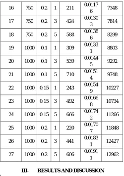
The experimental results of Thrust force, tool wear and simulation temperature for all the trails are tabulated in Table 3 as shown below.

Table 3 Responses for trials

Exp No S F D

Temper ature

(°C)

Tool Wear (mm)

Thrust Force (N)

1 500 0.1 1 246 0.0024

4 2280

2 500 0.1 3 499 0.0036

4 2572

3 500 0.1 5 695 0.0044 2818

4 500 0.15 1 178 0.0047

3 3111

5 500 0.15 3 437 0.0059

9 3369

6 500 0.15 5 615 0.0068 3707

7 500 0.2 1 156 0.0064

2 3987

8 500 0.2 3 390 0.0077

3 4360

9 500 0.2 5 561 0.0085

9 4682

10 750 0.1 1 259 0.0078

9 5001

11 750 0.1 3 524 0.0090

6 5379

12 750 0.1 5 699 0.0097

8 5727

13 750 0.15 1 216 0.0101

3 6099

14 750 0.15 3 461 0.0113

5 6511

15 750 0.15 5 618 0.0121

16 750 0.2 1 211 0.0117

6 7348

17 750 0.2 3 424 0.0130

3 7814

18 750 0.2 5 588 0.0138

6 8299

19 1000 0.1 1 309 0.0133

1 8803

20 1000 0.1 3 539 0.0144

5 9292

21 1000 0.1 5 710 0.0151

4 9748

22 1000 0.15 1 243 0.0154

9 10227

23 1000 0.15 3 492 0.0166

8 10734

24 1000 0.15 5 666 0.0174

2 11266

25 1000 0.2 1 220 0.0170

7 11848

26 1000 0.2 3 441 0.0183

1 12427

27 1000 0.2 5 606 0.0191

1 12962

III. RESULTS AND DISCUSSION A. Analysis of Variance (ANOVA)

Analysis of Variance is carried out on the obtained experimental data to check the significance of the model.

Table 4 Anova- temperature

Source Sum of

Squares df

Mean

Squares F Value p-value Model 833260.5278 9 92584.503 981.1722 <0.0001 A-s 11200.05556 1 11200.055 118.6935 <0.0001 B-f 43316.05556 1 43316.055 459.0456 <0.0001 C-d 768800.000 1 768800.00 8147.424 <0.0001

AB 147.000000 1 147.0000 1.557845 0.22890

AC 546.750000 1 546.7500 5.794230 0.02772

BC 1240.333333 1 1240.3333 13.14453 0.00209

A^2 0.166666667 1 0.166666 0.001766 0.96697

B^2 937.5000000 1 937.5000 9.935236 0.00582

C^2 7072.666667 1 7072.666 74.95319 <0.0001

Residual 1604.138889 17 94.36111

Cor

From the above analysis it was found that feed and depth of cut are the most significant terms affecting the Tool Temperature as their p-values are <0.0001. R2=0.9450 which is 94.5%. The desirable value is close to 1 which indicates that the model has a variance of 5.5% and hence is within the acceptable limits.

Table 5Anova- thrust force

Source Sum of Squares

d f

Mean

Squares F Value p-value

Model 2.79E+0

8 9

3.10E+0 7 7.74E+0 4 <0.000 1

A-s 2.45E+0

8 1

2.45E+0 8 6.12E+0 5 <0.000 1

B-f 2.72E+0

7 1

2.72E+0 7 6.78E+0 4 <0.000 1

C-d 3.09E+0

6 1

3.09E+0 6 7.72E+0 3 <0.000 1

AB 1.36E+0

6 1

1.36E+0 6 3.39E+0 3 <0.000 1

AC 1.34E+0

5 1

1.34E+0 5 3.35E+0 2 <0.000 1

BC 2.53E+0

4 1

2.53E+0 4 6.32E+0 1 <0.000 1

A^2 1.83E+0

6 1

1.83E+0 6 4.56E+0 3 <0.000 1

B^2 3.59E+0

4 1

3.59E+0 4 8.98E+0 1 <0.000 1

C^2 4.63E+0

1 1

4.63E+0 1 1.16E-01 0.7379 6 Residu al 6.80E+0 3 1 7 4.00E+0 2 Cor Total 2.79E+0 8 2 6

From the above analysis it was found that speed and feed are the most significant terms affecting the Tool Temperature as their p-values are <0.0001. R2=0.9546 which is 95.46%. The desirable value is close to 1 which indicates that the model has a variance of 4.54% and hence is within the acceptable limits

B. Principal Component Analysis (PCA) Integrated Taguchi Analysis

PCA is an optimisation tool which converts several multiple correlated responses into several uncorrelated quality indices. It maximises the variability of the data while minimizing the dimensionality of the data. The following steps are involved in the process.

1) Normalisation of data: The normalized values are calculated using the formula given below.

( ) = max ( )− ( )

Table 6 Normalised data Trial

No Temperature

Tool Wear

Thrust Force

1 0.837545 1 1

2 0.380866 0.928014 0.972664

3 0.027076 0.882424 0.949635

4 0.960289 0.862627 0.922206

5 0.49278 0.787043 0.898053

6 0.17148 0.738452 0.866411

7 1 0.761248 0.840198

8 0.577617 0.682663 0.80528

9 0.268953 0.631074 0.775136

10 0.814079 0.673065 0.745272

11 0.33574 0.602879 0.709886

12 0.019856 0.559688 0.677308

13 0.891697 0.538692 0.642483

14 0.449458 0.465507 0.603913

15 0.166065 0.419316 0.562535

16 0.900722 0.440912 0.525557

17 0.516245 0.364727 0.481932

18 0.220217 0.314937 0.436529

19 0.723827 0.34793 0.389347

20 0.308664 0.279544 0.343569

21 0 0.238152 0.30088

22 0.84296 0.217157 0.256038

23 0.393502 0.145771 0.208575

24 0.079422 0.10138 0.158772

25 0.884477 0.122376 0.104288

26 0.48556 0.04799 0.050084

27 0.187726 0 0

Table 7 Eigen values

PC1 PC2 PC3

Eigen Value 2.0428 0.9482 0.0091

Accountability Proportion

(AP)

0.681 0.316 0.003

TABLE 7 EIGEN VECTORS

0.221 0.974 0.041

0.693 -0.127 -0.71

0.687 -0.185 0.703

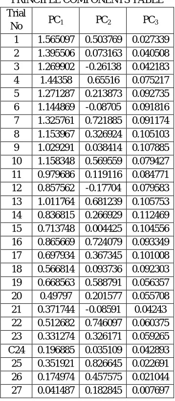
2) Calculating Principal Components (PC), Composite Principal Components (CPC) and S/N values: The principal components, Composite Principal components and S/N values are calculated from the following formulae.

PC1=(0.221*T)+(0.693*Tw)+(0.687*Tf)

PC2=(0.974*T)+(-0.127*Tw)+(-0.185*Tf)

PC3=(0.041*T)+(-0.71*Tw)+(0.703*Tf)

CPC = (PC12+PC22+PC32)1/3

=−10log₁₀1 1₂

1

Where is S/N Value and y is CPC Value

TABLE 8

PRINCIPLE COMPONENTS TABLE Trial

No PC1 PC2 PC3

1 1.565097 0.503769 0.027339

2 1.395506 0.073163 0.040508

3 1.269902 -0.26138 0.042183

4 1.44358 0.65516 0.075217

5 1.271287 0.213873 0.092735

6 1.144869 -0.08705 0.091816

7 1.325761 0.721885 0.091174

8 1.153967 0.326924 0.105103

9 1.029291 0.038414 0.107885

10 1.158348 0.569559 0.079427

11 0.979686 0.119116 0.084771

12 0.857562 -0.17704 0.079583

13 1.011764 0.681239 0.105753

14 0.836815 0.266929 0.112469

15 0.713748 0.004425 0.104556

16 0.865669 0.724079 0.093349

17 0.697934 0.367345 0.101008

18 0.566814 0.093736 0.092303

19 0.668563 0.588791 0.056357

20 0.49797 0.201577 0.055708

21 0.371744 -0.08591 0.04243

22 0.512682 0.746097 0.060375

23 0.331274 0.326171 0.059265

C24 0.196885 0.035109 0.042893

25 0.351921 0.826645 0.022691

26 0.174974 0.457575 0.021044

Table 9 Cpc and s/n values Trial

No CPC

S/N Value

1 1.393174 -2.88011

2 1.250278 -1.94013

3 1.189433 -1.5068

4 1.360605 -2.67464

5 1.186542 -1.48566

6 1.098823 -0.81855

7 1.317528 -2.3952

8 1.131738 -1.07492

9 1.023623 -0.2028

10 1.187007 -1.48907

11 0.99368 0.055072

12 0.91779 0.745131

13 1.144444 -1.17189

14 0.92215 0.70397

15 0.804345 1.891152 16 1.086442 -0.72013 17 0.858284 1.327378 18 0.696984 3.135549 19 0.927089 0.657574

20 0.66321 3.56698

21 0.528211 5.543856 22 0.937187 0.563476 23 0.603354 4.388554

24 0.34715 9.18966

25 0.931289 0.618312

26 0.62182 4.126703

27 0.327768 9.688675

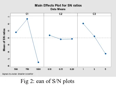
From the above analysis the mean of S/N values plot was obtained

Fig 2: ean of S/N plots

IV. CONCLUSION

The optimal values of Temperature, Tool wear and Thrust Force 666°C, 0.01742mm and 11266N respectively were obtained at a cutting speed of 1000 rpm, feed rate of 0.15 mm/rev, Drill depth of 5 mm.

1000 750 500 -1 -2 -3 -4 -5 -6 -7 -8 0.20 0.15

0.10 1 3 5

C1 M e a n o f S N r at io s C2 C3

Main Effects Plot for SN ratios

Data Means

REFERENCES [1] SFTC Deform 3D, V.6.1, Scientific Forming Technologies Corporation

[2] A.V. Mitrfanov, V.I. Babitsky, V.V. Silbersschmidt (2005), Finite element analysis of ultrasonicallyassisted turning of Inconel 718, journal of Materials Processing Technology, vol. 153–154, pp. 233–239.

[3] C.Z. Duan, T. Dou, Y.J. Cai, Y.Y. Li (2005), Finite Element Simulation and Experiment of Chipformation Process during High Speed Machining of AISI 1045 Hardened Steel, International Journal ofRecent Trends in Engineering, Vol. 5, pp. 46–50

[4] Design Expert Software, version 8, Users Guide, Technical Manual, Stat-Ease Inc.

[5] H.K. Kansal, Sehijpal Sing, P. Kumar (2005), Parametric optimization of powder mixed electricaldischarge machining by response surface methodology, Journal of Materials Processing Technology, vol.169, pp. 427–436.

[6] I.A. Choudary, M.A. El-Baradie (1999), Machinability assessment of Inconel 718 by factorial design ofexperiment coupled with response surface methodology, Journal of Material processing Technology vol.95, pp. 30–39.

[7] K. Kadirgama, M.M. Noor, M.M. Rahman, W.S.W. Harun, C.H.C. Haron (2009), Finite ElementAnalysis and Statistical Method to Determine Temperature Distribution on Cutting Tool in End-Milling, European Journal of Scientific Research, Vol. 30, No. 3, pp. 415–463.

[8] L. Filice, D. Umbrello, S. Beccari, F. Micari (2006), On the FE codes capability for tool temperaturecalculation in machining processes, Journal of Materials Processing Technology, vol. 174, pp. 286–292.

[9] RavirajShetty, Laxmikant K, R. Pai and S.S. Rao (2008), Finite element modeling of stress distributionin the cutting path in machining of discontinuously reinforced aluminium composites, ARPN Journal ofEngineering and Applied Sciences, Vol. 3, pp. 25–31.

[10] Rui Li, Albert J.Shih (2006), Finite element modeling of 3D turning of titanium, International Journalof Advanced Manufacturing Technology, vol. 29, pp. 253–261.

[11] A. Karabulut (2010), Determination of diametral error using finite element and experimental method, METABK, vol. 49(1), pp. 57–60

[12] Usui, E., Shirakashi, T. and Kitagawa, T. (1978), Analytical prediction of three dimensional cuttingprocess, part 3: cutting temperature and crater wear of carbide tool, Journal of Engineering for Industry,vol. 100 (5), pp. 236–243.