Thesis by
Alex Gittens
In Partial Fulfillment of the Requirements for the Degree of
Doctor of Philosophy
California Institute of Technology Pasadena, California
2013
Acknowledgements
I have been privileged to befriend and work with exceptional individuals.
I owe a debt of thank to Drs. Emmanuel Papadakis and Gordon Johnson of the University of Houston for helping me get started on my academic path. I consider myself lucky to have had the guidance of my PhD advisor, Joel Tropp, and remain humbled by his intuitive grasp of the ideas and tools I have wrestled with throughout my graduate career. In addition to Joel, I am grateful to the other collaborators I was privileged to work with: Christos Boutsidis, Michael Mahoney, and Richard Chen. It was a pleasure working with them.
I benefited greatly from interactions with my fellow students; in particular, I thank Catherine Beni, Chia-Chieh Chu, Derek Leong, Jinghao Huang, and Yamuna Phal for being great office mates and friends. My dear friend and amateur herpetologist Yekaterina Pavlova I thank for being her very unique self. Stephen Becker, Michael McCoy, Peter Stobbe, Patrick Sanan, Zhiyi Li, George Chen, and Yaniv Plan may have provided answers to the odd math question, but I appreciate them more for the hours of wide-ranging discussions on everything under the sun.
Abstract
This thesis studies three classes of randomized numerical linear algebra algorithms, namely: (i) randomized matrix sparsification algorithms, (ii) low-rank approximation algorithms that use randomized unitary transformations, and (iii) low-rank approximation algorithms for positive-semidefinite (PSD) matrices.
Randomized matrix sparsification algorithms set randomly chosen entries of the input matrix to zero. When the approximant is substituted for the original matrix in computations, its sparsity allows one to employ faster sparsity-exploiting algorithms. This thesis contributes bounds on the approximation error of nonuniform randomized sparsification schemes, measured in the spectral norm and two NP-hard norms that are of interest in computational graph theory and subset selection applications.
Low-rank approximations based on randomized unitary transformations have several desir-able properties: they have low communication costs, are amendesir-able to parallel implementation, and exploit the existence of fast transform algorithms. This thesis investigates the tradeoff between the accuracy and cost of generating such approximations. State-of-the-art spectral and Frobenius-norm error bounds are provided.
suite of canonical matrices drawn from machine learning and data analysis applications, and a framework is developed for establishing theoretical error bounds.
Contents
Acknowledgements iii
Abstract iv
List of Figures xi
List of Tables xiii
1 Introduction and contributions 1
1.1 The sampling approach to matrix approximation. . . 3
1.2 The random-projection approach to matrix approximation. . . 7
1.3 Nonasymptotic random matrix theory . . . 9
1.4 Contributions . . . 12
1.4.1 Nonasymptotic random matrix theory . . . 12
1.4.2 Matrix sparsification. . . 13
1.4.3 Low-rank approximation using fast unitary transformations . . . 16
1.4.4 Randomized SPSD sketches . . . 17
2 Bounds for all eigenvalues of sums of Hermitian random matrices 20 2.1 Introduction . . . 20
2.3 The Courant–Fisher Theorem. . . 22
2.4 Tail bounds for interior eigenvalues . . . 23
2.5 Chernoff bounds. . . 28
2.6 Bennett and Bernstein inequalities. . . 32
2.7 An application to column subsampling . . . 38
2.8 Covariance estimation . . . 41
2.8.1 Proof of Theorem 2.15 . . . 47
2.8.2 Extensions of Theorem 2.15 . . . 51
2.8.3 Proofs of the supporting lemmas . . . 53
3 Randomized sparsification in NP-hard norms 58 3.1 Notation. . . 60
3.1.0.1 Graph sparsification . . . 61
3.2 Preliminaries . . . 63
3.3 The∞→pnorm of a random matrix . . . 66
3.3.1 The expected∞→pnorm . . . 66
3.3.2 A tail bound for the∞→pnorm . . . 68
3.4 Approximation in the∞→1 norm . . . 70
3.4.1 The expected∞→1 norm . . . 70
3.4.2 Optimality . . . 72
3.4.3 An example application . . . 74
3.5 Approximation in the∞→2 norm . . . 75
3.5.1 Optimality . . . 78
3.6 A spectral error bound . . . 80
3.6.1 Comparison with previous results. . . 82
3.6.1.1 A matrix quantization scheme . . . 82
3.6.1.2 A nonuniform sparsification scheme . . . 83
3.6.1.3 A scheme which simultaneously sparsifies and quantizes . . . . 85
3.7 Comparison with later bounds . . . 86
4 Preliminaries for the investigation of low-rank approximation algorithms 89 4.1 Probabilistic tools. . . 89
4.1.1 Concentration of convex functions of Rademacher variables . . . 89
4.1.2 Chernoff bounds for sampling without replacement . . . 90
4.1.3 Frobenius-norm error bounds for matrix multiplication . . . 91
4.2 Linear Algebra notation and results . . . 96
4.2.1 Column-based low-rank approximation. . . 98
4.2.1.1 Matrix Pythagoras and generalized least-squares regression . . . 99
4.2.1.2 Low-rank approximations restricted to subspaces . . . 100
4.2.2 Structural results for low-rank approximation . . . 101
4.2.2.1 A geometric interpretation of the sampling interaction matrix . . 102
5 Low-rank approximation with subsampled unitary transformations 105 5.1 Introduction . . . 105
5.2 Low-rank matrix approximation using SRHTs . . . 110
5.2.1 Detailed comparison with prior work . . . 111
5.3 Matrix computations with SRHT matrices . . . 118
5.3.2 SRHTs applied to general matrices . . . 123
5.4 Proof of the quality of approximation guarantees . . . 132
5.5 Experiments . . . 142
5.5.1 The test matrices . . . 143
5.5.2 Empirical comparison of the SRHT and Gaussian algorithms . . . 146
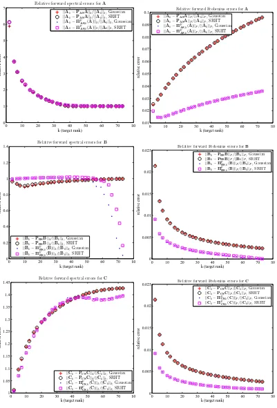
5.5.3 Empirical evaluation of our error bounds . . . 147
6 Theoretical and empirical aspects of SPSD sketches 153 6.1 Introduction . . . 153
6.1.1 Outline . . . 156
6.2 Deterministic bounds on the errors of SPSD sketches . . . 157
6.3 Comparison with prior work . . . 162
6.4 Proof of the deterministic error bounds. . . 164
6.4.1 Spectral-norm bounds. . . 165
6.4.2 Frobenius-norm bounds . . . 168
6.4.3 Trace-norm bounds . . . 173
6.5 Error bounds for Nyström extensions . . . 175
6.6 Error bounds for random mixture-based SPSD sketches. . . 181
6.6.1 Sampling with leverage-based importance sampling probabilities . . . 182
6.6.2 Random projections with subsampled randomized Fourier transforms . . 185
6.6.3 Random projections with i.i.d. Gaussian random matrices . . . 188
6.7 Stable algorithms for computing regularized SPSD sketches . . . 192
6.8.2 Dependence on coherence . . . 198
6.9 Empirical aspects of SPSD low-rank approximation . . . 201
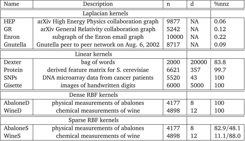
6.9.1 Test matrices . . . 202
6.9.2 A comparison of empirical errors with the theoretical error bounds. . . 207
6.9.3 Reconstruction accuracy of sampling and projection-based sketches . . . . 209
6.9.3.1 Graph Laplacians . . . 209
6.9.3.2 Linear kernels . . . 216
6.9.3.3 Dense and sparse RBF kernels . . . 219
6.9.3.4 Summary of comparison of sampling and mixture-based SPSD Sketches . . . 225
6.10 A comparison with projection-based low-rank approximations . . . 226
List of Figures
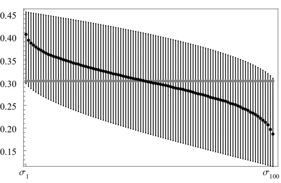
2.1 Spectrum of a random submatrix of a unitary DFT matrix.. . . 41
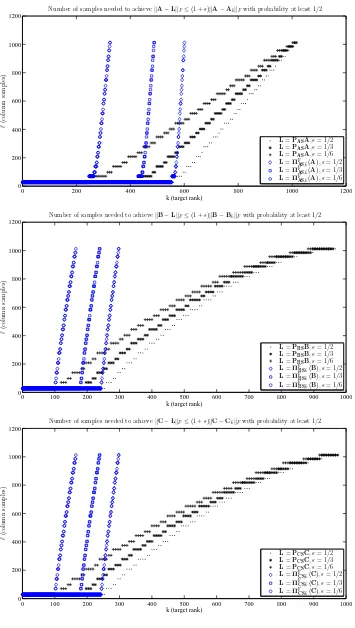
5.1 Residual errors of low-rank approximation algorithms . . . 145 5.2 Forward errors of low-rank approximation algorithms . . . 148 5.3 The number of column samples required for relative error Frobenius-norm
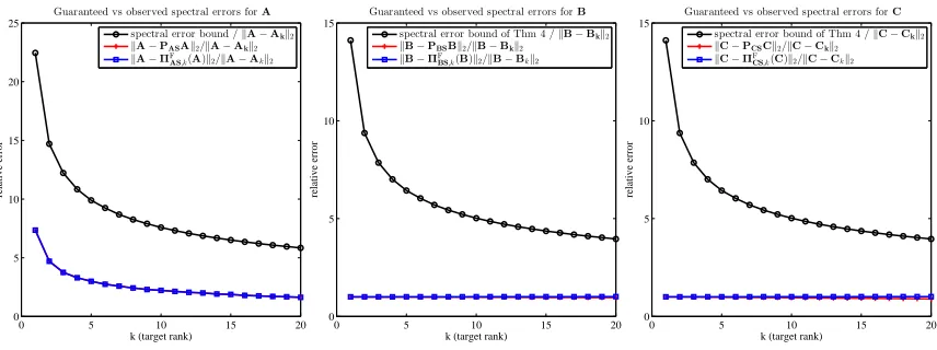
approxi-mations . . . 149 5.4 Empirical versus predicted spectral-norm residual errors of low-rank approximations152
6.1 Empirical demonstration of the optimality of Theorem 6.9. . . 198 6.2 Spectral-norm errors of regularized Nyström extensions as coherence varies. . . . 200 6.3 Spectral-norm error of regularized Nyström extensions as regularization parameter
varies . . . 202 6.4 Relative errors of non-rank-restricted SPSD sketches of the GR and HEP Laplacian
matrices. . . 210 6.5 Relative errors of non-rank-restricted SPSD sketches of the Enron and Gnutella
Laplacian matrices . . . 211 6.6 Relative errors of rank-restricted SPSD sketches of the GR and HEP Laplacian matrices212
6.7 Relative errors of rank-restricted SPSD sketches of the Enron and Gnutella Laplacian
6.8 Relative errors of non-rank-restricted SPSD sketches of the linear kernel matrices . 217 6.9 Relative errors of rank-restricted SPSD sketches of the linear kernel matrices . . . 218 6.10 Relative errors of non-rank-restricted SPSD sketches of the dense RBFK matrices . 220 6.11 Relative errors of rank-restricted SPSD sketches of the dense RBFK matrices. . . 221 6.12 Relative errors of non-rank-restricted SPSD sketches of the sparse RBFK matrices . 222 6.13 Relative errors of rank-restricted SPSD sketches of the sparse RBFK matrices . . . 223 6.14 Comparison of projection-based low-rank approximations with one-pass SPSD
List of Tables
6.1 Asymptotic comparison of our bounds on SPSD sketches with prior work . . . 163
6.2 Information on the SPSD matrices used in our empirical evaluations . . . 203
6.3 Statistics of our test matrices . . . 205
Chapter 1
Introduction and contributions
require multiple passes over the matrix, which may incur high communication costs if the matrix is stored in a distributed fashion, or if the data has to percolate through a hierarchical memory architecture[CW09].
Much interest has been expressed in finding o(kn2)low-rank approximation schemes that offer approximation guarantees comparable with those of the truncated SVD. Randomized numerical linear algebra(RNLA) refers to a field of research that arose in the early 2000s at the intersection of several research communities, including the theoretical computer science and numerical linear algebra communities, in response to the desire for fast, efficient algorithms for manipulating large matrices. RNLA algorithms for matrix approximation focus on reducing the number of arithmetic operations and the communications costs of algorithms by judiciously exploiting randomness. Typically, these algorithms take one of two approaches. The sampling approach advocates using information obtained by randomly sampling the columns, rows, or entries of the matrix to form an approximation to the matrix. The random projection approach randomly mixes the entries of the matrix before employing the sampling approach. The analysis of both classes of algorithms requires the use of tools from the nonasymptotic theory of random matrices.
This thesis contributes to both approaches to forming randomized matrix approximants, and it extends the toolset available to researchers working in the field of RNLA.
• Chapter2builds upon the matrix Laplace transform originated by Ahlswede and Winter to provide eigenvalue analogs of classical exponential tail bounds foralleigenvalues of a sum of random Hermitian matrices. Such sums arise often in the analysis of RNLA algorithms.
entry-wise sparsification algorithms.
• Chapter5provides guarantees on the quality of low-rank approximations generated using a class of random projections that exploit fast unitary transformations.
• Chapter6concludes by providing a framework for the analysis of a diverse class of low-rank approximations to positive-semidefinite matrices, as well as empirical evidence of the efficacy of these approximations over a wide range of matrices. The class of approximations considered includes both sampling-based approximations as well as projection-based approximations.
In the remainder of this introductory chapter, we survey the sampling and projection-based approaches to randomized matrix approximation and the tools currently available to researchers for the interrogation of the properties of random matrices. We conclude with an overview of the contributions of this thesis.
1.1
The sampling approach to matrix approximation
Sparse approximants are of interest because they be used in lieu of the original matrix to reduce the cost of calculations. Randomized sparsified approximations to matrices have found applications in approximate eigenvector computations[AM01,AHK06,AM07]and semidefinite optimization algorithms[AHK05,d’A11].
work, they presented a scheme that randomly quantizes the entries of the matrix to±maxi j|Ai j|.
Such quantization schemes are of interest because they reduce the cost of storing and working with the matrix. Note that this quantization scheme requires two passes over the matrix: one to computeb, then another to quantize. The bounds given in[AM07]for both schemes guarantee that the spectral norm error of the approximations to a matrixA∈Rm×n remain on the order ofpmax{m,n}maxi j|Ai j|with high probability. If each entry in the matrix is replaced by zero with probability 1−p, the expected number of nonzeros in the approximant is shown to be at mostpkAk2F/maxi j|Ai j|2+4096mlog4(n). These bounds are quite weak: the algorithms perform much better on average.
Arora et al. presented an alternative quantization and sparsification scheme in[AHK06]that has the advantage of requiring only one pass over the input matrix. The schemes of both Arora et. al and Achlioptas and McSherry involve entrywise calculations on the matrix being approximated, and have the property that the entries in the random approximant are independent of each other. Succeeding works on entry-wise matrix sparsification include[NDT10,DZ11,AKL13]; the algorithms given in these works also produce approximants with independent entries. The sharpest available bound on randomized element-wise sparsification is satisfied by the algorithm given in[DZ11]: given an accuracy parameterε >0, this algorithm produces an approximant that satisfieskA−A˜k2≤εwith high probability and has at most 28ε2nlog(p2n)kAk2Fnonzero entries; the approximant can be calculated in one pass. The paper[NDT10]goes beyond matrix sparsification, addressing randomized element-wise tensor sparsification.
propose judiciously sampling a submatrix fromAand using the SVD of this submatrix to find an approximation of the top singular spaces ofA. The projection ofAonto this subspace is then used as the low-rank approximation. This algorithm of course requires two passes over the matrix. The original idea in[FKV98]was refined in a series of papers providing increasingly strong guarantees on the quality of the approximation[DK01,DK03,FKV04,DKM06a,DKM06b].
Rudelson and Vershynin take a different approach to the analysis of the Monte Carlo methodology for low-rank approximation in [RV07]. They consider A as a linear operator between finite-dimensional Banach spaces and apply techniques of probability in Banach spaces: decoupling, symmetrization, Slepian’s lemma for Rademacher random variables, and a law of large numbers for operator-valued random variables. They show that, ifAhas numerical rank close tok, then it is possible to obtain an accurate rank-kapproximation toAby sampling O klogk
rows ofA. Specifically, if one projects Aonto the span of`=O(ε−4klogk) of its rows, then the approximant satisfieskA−A˜k2≤ kA−Akk2+εkAk2 with high probability. Here
Akdenotes the optimal rank-kapproximation toA, obtainable as the rank-ktruncated SVD ofA. Other researchers forwent the SVD entirely, considering instead alternative column and row-based matrix decompositions. In one popular class of approximations, the matrix is approximated with a product CUR, whereCand Rare respectively small subsets of the columns and rows of the matrix andU, the coupling matrix, is computed fromCandR[DKM06c]. Accordingly, these schemes are known as CUR decompositions. Nyström extensions, introduced by Williams and Seeger in[WS01], are a similar class of low-rank approximations to positive-semidefinite matrices. They can be thought of as CUR decompositions constructed with the additional constraint thatC=RT, to preserve the positive-semidefiniteness of the approximant. Both CUR and Nyström decompositions can be constructed in one pass over the matrix.
rows to formCandRand showed that approximations formed with O(klogk)columns and rows in this manner achieve Frobenius norm errors close to the optimal rank-kapproximation error:
kA−CURkF≤(1+")kA−AkkF. Theleverage scoresof the columns ofAare used to generate
the probability distribution used for column sampling: givenP, a projection onto the dominant k-dimensional right singular space ofA, the leverage score of the jth column ofAis proportional to(P)ii. The intuition is that the magnitude of the leverage score of a particular column reflects its influence in determining the dominantk-dimensional singular spaces ofA[DM10].
In[MRT06,MRT11], Tygert et al. introduced randomized Interpolative Decompositions (ID) as an alternative low-rank factorization to the SVD. In IDs, the columns ofAare represented as linear combinations of some small subset of the columns ofA. The algorithm of[MRT06]
is accelerated in [WLRT08]. With high probability, it constructs matricesB andΠsuch that
Bconsists of kcolumns sampled fromA, some subset of the columns ofΠmake up thek×k identity matrix, andkA−BΠk2=O(pkmnkA−Akk2).
The works of Har-Peled [HP06], and Deshpande et al.[DRVW06]use more intricate ap-proaches based on column sampling to produce low-rank approximations with relative-error Frobenius norm guarantees. These algorithms require, respectively, O(k2logk)and O(k)column samples.
they demonstrate the existence of a matrixAsuch that
kA−A˜k2≥ 1+
r
n2+α
`2+α
!
kA−Akk2
when ˜Aisanyapproximation obtained by projectingAonto the span of`of its columns. Because this bound holds regardless of how the columns are selected, it is clear that, at least in the spectral norm, the sampling paradigm is not sufficient to obtain near optimal approximation errors. Stronger spectral norm guarantees can be obtained using the random projection approach to matrix approximation.
1.2
The random-projection approach to matrix approximation
A wide range of results in RNLA have been inspired by the work of Johnson and Lindenstrauss in geometric functional analysis, who showed that embeddings into random low-dimensional spaces can preserve the geometry of point sets. The celebrated Johnson–Lindenstrauss lemma states that, given npoints in a high-dimensional space, a random projection into a space of dimension Ω(logn) preserves the distance between the points. Such geometry-preserving, dimension-reducing maps are known as Johnson–Lindenstrauss transforms (JLT).
The work of Papadimitriou et al. in[PRTV00]on the algorithmic application of randomness to facilitate information retrieval popularized the use of JLTs in RNLA. Unlike sample-based methods like the CUR decomposition that project the matrix onto the span of a subset of its
One then obtains a low-rank approximation of the matrix by projecting it onto this approximate singular space. Projection-based matrix approximation algorithms require at least two passes over the matrix: one to form an approximate basis for the top left singular space of the matrix, and one to project the matrix onto that basis.
In the influential paper[Sar06], Sarlós developed fast approximation algorithms for SVDs, least squares, and matrix multiplication under the randomized projection paradigm. His algo-rithms take advantage of Ailon and Chazelle’s work, which establish that certain structured randomized transformations can be used to quickly compute dimension reductions[AC06]. At around the same time, Martinsson, Rohklin, and Tygert introduced a randomized projection-based algorithm for the calculation of approximate SVDs[MRT06,MRT11]. In this algorithm, to obtain an approximate rank-kSVD ofA, one appliesk+pgaussian vectors toAthen projects
Aonto the resulting subspace. Here,pis a small integer known as theoversampling parameter. The approximation returned by the algorithm can be written as ˜A=PASA, whereSis a Gaussian matrix and the notationPMdenotes the projection onto the range of the matrixM. The spectral norm error of the approximant is guaranteed to be at most pmaxm,nkA−Akk2 with high probability, and ifAis unstructured and dense, the algorithm costs O(mnk)time. Despite the fact that its runtime is asymptotically the same as those of classical Krylov iteration schemes (e.g. the Lanczos method), this algorithm is of interest because it requires only two passes over the matrix. Moreover, the algorithm performs well in the presence of degenerate singular values, a situation which often causes Lanczos methods to stagnate[MRT11]. Finally, this algorithm is more readily parallelizable than iterative schemes.
they show that if the “sampling matrix”Sconsists of O(k2)uniformly randomly selected columns of the product of the discrete Fourier transform matrix and a diagonal matrix of random signs, then the error guarantees of the algorithm remain unchanged while the worst-case runtime decreases. Nguyen et al. consider the same approximation in[NDT09], ˜A=PASA, and obtain improved results: ifShas O(klogk)columns constructed as in the algorithm of[WLRT08], then with constant probabilitykA−A˜k2≤p
m/(klogk)kA−Akk2.
The paper[BDMI11]and the survey article[HMT11]constituted a significant step forward in the analysis of random projection-based matrix approximation algorithms, because they provided a framework for the analysis of the Frobenius and spectral norm errors of approximants of the formPASAusing arbitrary sampling matricesS. In[HMT11], this framework is used to provide guarantees on the errors of approximants of the form ˜A=PASAforSGaussian and for
Sconsisting of uniformly randomly selected columns of the product of the Walsh–Hadamard transform matrix and a diagonal matrix of random signs.
1.3
Nonasymptotic random matrix theory
generality, the sparsification algorithms became more sophisticated, and the analysis of their errors became sharper.
The study of the spectra of random matrices is naturally divided into two subfields: the nonasymptotic theory, which gives probability bounds that hold for finite-dimensional matrices but may not be sharp, and the asymptotic theory, which precisely describes the behavior of certain families of matrices as their dimensions go to infinity. Unfortunately, the strength of the asymptotic techniques lies in the determination of convergence and the development of asymptotically sharp bounds, rather than the development of tail bounds which hold at a fixed dimension. Accordingly, the nonasymptotic theory is of most relevance in RNLA applications.
The sharpest and most comprehensive results available in the nonasymptotic theory concern the behavior of Gaussian matrices. The amenability of the Gaussian distribution makes it possible to obtain results such as Szarek’s nonasymptotic analog of the Wigner semicircle theorem for Gaussian matrices [Sza90] and Chen and Dongarra’s bounds on the condition number of Gaussian matrices[CD05]. The properties of less well-behaved random matrices can sometimes be related back to those of Gaussian matrices using probabilistic tools, such as symmetrization; see, e.g., the derivation of Latała’s bound on the norms of zero-mean random matrices[Lat05]. More generally, bounds on extremal eigenvalues can be obtained from knowledge of the moments of the entries. For example, the smallest singular value of a square matrix with i.i.d. zero-mean subgaussian entries is O(n−1/2) with high probability[RV08]. Concentration of measure results, such as Talagrand’s concentration inequality for product spaces [Tal95], have also contributed greatly to the nonasymptotic theory. We mention in particular the work of Achlioptas and McSherry on randomized sparsification of matrices[AM01,AM07], that of Meckes on the norms of random matrices[Mec04], and that of Alon, Krivelevich and Vu[AKV02]
applications of Talagrand’s inequality. In cases where geometric information on the distribution of the random matrices is available, the tools of empirical process theory—such as generic chaining, also due to Talagrand[Tal05]—can be used to convert this geometric information into information on the spectra. One natural example of such a case consists of matrices whose rows are independently drawn from a log-concave distribution[MP06,ALPTJ11].
One of the most general tools in the nonasymptotic theory toolbox is the Noncommutative Khintchine Inequality (NCKI), which bounds the moments of the norm of a sum of randomly signed matrices[LPP91]. Despite its power and generality, the NCKI is unwieldy. To use it, one must reduce the problem to a suitable form by applying symmetrization and decoupling arguments and exploiting the equivalence between moments and tail bounds. It is often more convenient to apply the NCKI in the guise of a lemma, due to Rudelson[Rud99], that provides an analog of the law of large numbers for sums of rank-one matrices. This result has found many applications, including column-subset selection[RV07]and the fast approximate solution of least-squares problems[DMMS11]. The NCKI and its corollaries do not always yield sharp results because parasitic logarithmic factors arise in many settings.
showed that these matrix probability inequalities can be sharpened considerably by working with cumulant generating functions instead of mgfs[Tro12,Tro11c,Tro11a].
Chatterjee established that in the scalar case, powerful concentration inequalities could be recovered from arguments based on the method of exchangeable pairs[Cha07]. Mackey and collaborators extended the method of exchangeable pairs to matrix-valued functions[MJC+12]. The resulting bounds are sufficiently sharp to recover the NCKI, and can even be used to interrogate the behavior of matrix-valued functions of dependent random variables. Most recently, Paulin et al. have further extended the matrix method of exchangeable pairs to apply to an even larger class of matrix-valued functions[PMT13].
Despite the diversity of the tools mentioned here, all share a common limitation: they provide bounds only on the extremal eigenvalues of the relevant classes of random matrices.
1.4
Contributions
We conclude with a summary of the main contributions of this thesis.
1.4.1
Nonasymptotic random matrix theory
The matrix Laplace transform technique pioneered by Ahlswede and Winter, which applies to sums of independent random matrices[AW02,Tro12], is one of the most generally applicable techniques in the arsenal of nonasymptotic random matrix theory.
class of random matrices.
The minimax Laplace transform introduced in Chapter2relates the behavior of thek-th eigenvalue of a random self-adjoint matrix to the behavior of its compressions to subspaces:
Pλk(Y)≥t ≤ inf θ>0minV
e−θt·Etr exp
eθV∗YV
where the minimization is taken over an appropriate set of matricesVwith orthonormal columns. We show that when one has sufficiently strong semidefinite bounds on the matrix cumulant generating functions logEeθV∗XiV of the compressions of the summandsX
i, the minimax Laplace
transform technique yields exponential probability bounds for all the eigenvalues ofY=PiXi. We employ the minimax Laplace transform to produce eigenvalue Chernoff, Bennett, and Bernstein bounds. As an example of the efficacy of this technique, we use the Chernoff bounds to find new bounds on the interior eigenvalues of matrices formed by sampling columns from matrices with orthonormal rows. We also demonstrate that our Bernstein bounds are powerful enough to recover known estimates on the number of samples needed to accurately estimate the eigenvalues of the covariance matrix of a Gaussian process by the eigenvalues of the sample covariance matrix. In the process of doing so, we provide novel results on the convergence rate of the individual eigenvalues of Gaussian sample covariance matrices.
1.4.2
Matrix sparsification
on approximations that have these properties[AM01,AHK06,AM07]. A generic framework for the analysis of such approximation schemes is established, and this essentially recapitulates the known guarantees for the referenced algorithms.
We show that the spectral norm approximation error of such schemes can be controlled in terms of the variances and fourth moments of the entries ofXas follows:
EkA−Xk2≤C
max
j
X
k
Var(Xjk)
1/2
+max
k
X
j
Var(Xjk)
1/2 X
jk
E(Xjk−ajk)4
1/4
, (1.4.1)
where C is a universal constant. This expectation bound is obtained by leveraging work done by Latała on the spectral norm of random matrices with zero mean entries[Lat05]. When the entries ofAare bounded (so that the variances of the entries ofXare small), an argument based on a bounded difference inequality shows that the approximation error does not exceed this expectation by much.
Inequality (1.4.1) identifies properties desirable in randomized approximation schemes: namely, that they minimize the maximum column and row norms of the variances of the entries, as well as the fourth moments of all entries. Thus our results supply guidance in the design of future approximation schemes. The results also yield comparable analyses of the quantization and sparsification schemes introduced in [AM01, AM07] and recover error bounds for the quantization/sparsification scheme proposed by Arora, Hazan, and Kale in[AHK06]that are comparable to those supplied in[AHK06]. However, for the more recent sparsification schemes presented in[NDT10, DZ11, AKL13], our results do not provide sparsification guarantees as strong as those offered in the originating papers.
measured using non-unitary invariant norms. The literature on randomized matrix approxima-tion has, with few excepapproxima-tions, focused on the behavior of the spectral and Frobenius norms. However, depending on the application, other norms are of more interest; for instance, the p→qnorms naturally arise when one considersAas a map from`p(Rn)to`
q(Rm). Consider, in
particular, the∞ →1 and∞ →2 norms, both of which are NP-hard to compute. The∞ →1 norm has applications in graph theory and combinatorics. The∞ →2 norm has applications in numerical linear algebra. In particular, it is a useful tool in the column subset selection problem: that of, given a matrixAwith unit norm columns, choosing a large subset of the columns ofAso that the resulting submatrix has a norm smaller than some fixed constant (larger than one).
In a similar way that sparsification can assist in applications where the spectral norm is relevant, we believe it can be of assistance in applications such as these where the norm of interest is ap→qnorm. Our main result is a bound on the expected∞ →pnorm of random matrices whose entries are independent and have mean zero:
EkZk∞→p≤2E
X
k"kzk
p+2 maxkukq=1E
X
k
X
j"jZjkuj
.
Here"is a vector of i.i.d. random signs, zk is the kth column ofZ, andp−1+q−1=1. This
implies the following bounds on the∞ →1 and∞ →2 norms:
EkZk∞→1≤2E(kZkcol+
ZT
col) and EkZk∞→2≤2EkZkF+2 min
D E
ZD−1
2→∞,
of the matrix. As in the case of the spectral norm, a bounded differences inequality guarantees that if the entries ofAare bounded, then the errorskA−Xk∞→ξforξ∈ {1, 2}concentrate about these expectations. Thus we have bounds on norms which are NP-hard to compute, in terms of much simpler quantities. Both these bounds are optimal in the sense that each term in the bound can be shown to be necessary. In the case of the∞ →1 norm, a matching lower bound establishes the sharpness of the bound.
1.4.3
Low-rank approximation using fast unitary transformations
Chapter 5offers a new analysis of the subsampled randomized Hadamard transform (SRHT) approach to low-rank approximation. This is a specific instance of a class of low-rank approxima-tion algorithms based on fast unitary transformaapproxima-tions, and the analysis provided applies,mutatis mutandis, to other low-rank approximation algorithms which use fast unitary transformations.
Let` >k be a positive integer and letS∈Rn×` be a matrix whose columns are random
vectors, then projection methods approximateAwith PASA, which has rank at most`. Here,
the notationPM denotes the projection onto the range ofM. One can reduce the cost of the algorithm by using random matricesSwhose structure allows for fast multiplication. Specifically, one can reduce the cost of forming the productASfrom O(mn`)to O(mnlog`). One choice of a structured random matrix is the transpose of the subsampled randomized Hadamard transform (SRHT),
S=
Ç
n
`·DH
TRT.
Here,Dis a diagonal matrix whose entries are independent random uniformly distributed signs,
Hadamard matrix; other orthogonal transforms whose entries are on the order ofn−1/2can be used as well, such as the discrete cosine transform or the discrete Hartley transform.
The previous tightest bound on the spectral-norm error of SRHT-based low-rank approxima-tions is given in[HMT11], where it is shown that
A−PASA
2≤
1+
Ç
7n
`
A−Ak
2
with probability at least 1−O(1/k)when`is at least on the order ofklogk. In some situations, this bound is close to optimal. But whenAis rank-deficient or has fast spectral decay, this result does not reflect the correct behavior. In Chapter5we establish that
A−PASA
2≤O
r
log(n)log(rank(A))
`
! A−Ak
2+O
r
log(rank(A))
`
! A−Ak
F
with constant failure probability. The factor in front of the optimal error has been reduced at the cost of the introduction of a Frobenius term. This Frobenius term is small whenAhas fast spectral decay. We also find Frobenius-norm error bounds.
1.4.4
Randomized SPSD sketches
Chapter6considers the problem of forming a low-rank approximation to a symmetric positive-semidefinite matrixA∈Rn×n using “SPSD sketches.” LetS be a matrix of size n×`, where
`n. Then the SPSD sketch ofAcorresponding toSisCW†CT, where
C=AS and W=STAS.
positive-semidefinite. The simplest such SPSD sketches are formed by taking S to contain random columns sampled uniformly without replacement from the appropriate identity matrix. These sketches, known as Nyström extensions, are popular in applications where it is expensive or undesirable to have full access toA: Nyström extensions require only knowledge of`columns ofA.
The accuracy of SPSD sketches can be increased using the so-called power method, wherein one takes the sketching matrix to beS=ApS
0 for some integer p≥ 2 andS0 is a sketching matrix. The corresponding SPSD sketch isApS0(S0TA2p−1S0)†ST0Ap.
Chapter6establishes a framework for the analysis of SPSD sketches, and supplies spectral, Frobenius, and trace-norm error bounds for SPSD sketches corresponding to randomSsampled from several distributions. The error bounds obtained are asymptotically smaller than the other bounds available in the literature for SPSD sketching schemes. Our bounds apply to sketches constructed using the power method, and we see that the errors of these sketches decrease like (λk+1(A)/λk(A))p.
In particular, our framework supplies an optimal spectral-norm error bound for Nyström extensions. Because they are based on uniform column sampling, Nyström extensions perform best when the information in the topk-dimensional eigenspace is distributed evenly throughout the columns ofA. One way to quantify this idea uses the concept ofcoherence, taken from the matrix completion literature[CR09]. LetS be ak-dimensional subspace ofRn. The coherence ofS is
µ(S) = n
kmaxi(PS)ii.
columns have essentially the same influence; ifµis large, then it is possible that there is a single column inAwhich alone determines one of the topkeigenvectors ofA.
Talwalkar and Rostamizadeh were the first to use coherence in the analysis of Nyström extensions. Let A be exactly rank-k and µ denote the coherence of its top k-dimensional eigenspace. In[TR10], they show that if one samples on the order ofµklog(k/δ)columns to form a Nyström extension, then with probability at least 1−δthe Nyström extension isexactly
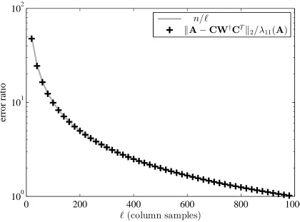
A. The framework provided in Chapter6allows us to expand this result to apply to matrices with arbitrary rank. Specifically, we show that when`=O(µklogk), then
A−CW†CT
2≤
1+n
`
A−Ak
2.
with constant probability. This bound is shown to be optimal in the worst case.
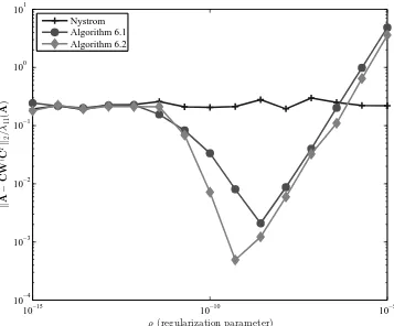
Low-rank approximations computed using the SPSD sketching model arenotguaranteed to be numerically stable: if Wis ill-conditioned, then instabilities may arise in forming the product CW†CT. A regularization scheme proposed in[WS01] suggests avoiding numerical ill-conditioning issues by using an SPSD sketch constructed from the matrixA+ρI, where
ρ >0 is a regularization parameter. In Chapter6, we provide the first error analysis of this
regularization scheme, and compare it empirically to another regularization scheme introduced in[CD11].
Chapter 2
Bounds for all eigenvalues of sums of
Hermitian random matrices
2.1
Introduction
The classical tools of nonasymptotic random matrix theory can sometimes give quite sharp estimates of the extreme eigenvalues of a Hermitian random matrix, but they are not readily adapted to the study of the interior eigenvalues. This is because, while the extremal eigenvalues are the maxima and minima of a random process, more delicate and challenging minimax problems must be solved to obtain the interior eigenvalues.
This chapter introduces a simple method, based upon the variational characterization of eigenvalues, that parlays bounds on the extreme eigenvalues of sums of random Hermitian matrices into bounds that apply to all the eigenvalues1. This technique extends the matrix Laplace transform method detailed in[Tro12]. We combine these ideas to extend several of the inequalities in[Tro12]to address the fluctuations of interior eigenvalues. Specifically, we provide eigenvalue analogs of the classical multiplicative Chernoff bounds and Bennett and Bernstein inequalities.
In this technique, the delicacy of the minimax problems which implicitly define the
ues of Hermitian matrices is encapsulated in terms that reflect the fluctuations of the summands in the appropriate eigenspaces. In particular, we see that the fluctuations of thekth eigenvalue of the sum above and below thekth eigenvalue of the expected sum are controlled by two different quantities. This satisfies intuition: for instance, given samples from a nondegenerate stationary random process with finite covariance matrix, one expects that the smallest eigenvalue of the sample covariance matrix is more likely to be an underestimate of the smallest eigenvalue of the covariance matrix than it is to be an overestimate.
We provide two illustrative applications of our eigenvalue tail bounds: Theorem 2.14 quantifies the behavior of the singular values of matrices obtained by sampling columns from a short, fat matrix; and Theorem2.15quantifies the convergence of the eigenvalues of Wishart matrices.
2.2
Notation
We defineMnsato be the set of Hermitian matrices with dimensionn. We often compare Hermitian matrices using the semidefinite ordering. In this ordering,Ais greater than or equal toB, written
ABorBA, whenA−Bis positive semidefinite.
The eigenvalues of a matrixAinMnsaare arranged in weakly decreasing order: λmax(A) =
λ1(A)≥λ2(A)≥ · · · ≥λn(A) =λmin(A). Likewise, the singular values of a rectangular matrixA
2.3
The Courant–Fisher Theorem
In this chapter, we work over the complex fieldC. One of our central tools is the variational characterization of the eigenvalues of a Hermitian matrix given by the Courant–Fischer Theorem. For integersdandnsatisfying 1≤d≤n, the complex Stiefel manifold
Vnd ={V∈C
n×d :V∗V=I}
is the collection of orthonormal bases for thed-dimensional subspaces ofCn, or, equivalently, the collection of all isometric embeddings of Cd intoCn. LetA be a Hermitian matrix with dimensionn, and letV∈Vn
d be an orthonormal basis for a subspace ofC
n. Then the matrix
V∗AVcan be interpreted as the compression ofAto the space spanned byV.
Proposition 2.1(Courant–Fischer ([HJ85, Theorem 4.2.11])). LetAbe a Hermitian matrix with dimension n. Then
λk(A) = min
V∈Vnn−k+1
λmax V∗AV
and (2.3.1)
λk(A) =max
V∈Vnk
λmin V∗AV
. (2.3.2)
A matrixV−∈Vnkachieves equality in(2.3.2)if and only if its columns span a top k-dimensional invariant subspace ofA.Likewise, a matrixV+∈Vnn−k+1 achieves equality in(2.3.1)if and only if its columns span a bottom(n−k+1)-dimensional invariant subspace ofA.
techniques we develop for bounding the eigenvalues from above to bound them from below.
2.4
Tail bounds for interior eigenvalues
In this section we develop a generic bound on the tail probabilities of eigenvalues of sums of independent, random, Hermitian matrices. We establish this bound by supplementing the matrix Laplace transform methodology of[Tro12]with Proposition2.1and a result, due to Lieb and Seiringer[LS05], on the concavity of a certain trace function on the cone of positive-definite matrices.
First we observe that the Courant–Fischer Theorem allows us to relate the behavior of thekth eigenvalue of a matrix to the behavior of the largest eigenvalue of an appropriate compression of the matrix.
Theorem 2.2. LetYbe a random Hermitian matrix with dimension n,and let k≤n be an integer. Then, for all t∈R,
Pλk(Y)≥t ≤ inf
θ>0 V∈minVnn−k+1
¦
e−θt·Etr eθV∗YV
©
. (2.4.1)
Proof. Letθ be a fixed positive number. Then
Pλk(Y)≥t =P
λk(θY)≥θt =P
¦
eλk(θY)≥eθt©
≤e−θt·Eeλk(θY)=e−θt·Eexp
¨
min
V∈Vnn−k+1
λmax θV∗YV
«
.
inequality and (2.3.1).
To continue, we need to bound the expectation. Use monotonicity to interchange the order of the exponential and the minimum; then apply the spectral mapping theorem to see that
Eexp
min
V∈Vnn−k+1
λmax θV∗YV
=E min
V∈Vnn−k+1
λmax exp(θV∗YV)
≤ min
V∈Vnn−k+1
Eλmax exp(θV∗YV)
≤ min
V∈Vnn−k+1
Etr exp(θV∗YV).
The first inequality is Jensen’s. The second inequality follows because the exponential of a Hermitian matrix is positive definite, so its largest eigenvalue is smaller than its trace.
Combine these observations and take the infimum over all positive θ to complete the argument.
In most cases it is prohibitively difficult to compute the quantity Etr eθV∗YV exactly. The main contribution of[Tro12]is a bound on this quantity, whenV=I, in terms of the cumulant generating functions of the summands. The main tool in the proof is a classical result due to Lieb[Lie73, Thm. 6]that establishes the concavity of the function
A7−→tr exp H+log(A)
(2.4.2)
on the positive-definite cone, whereHis Hermitian.
We are interested in the case whereV6=Iand the matrixYin Theorem2.2can be expressed as a sum of independent random matrices. In this case, we use the following result to develop the right-hand side of the Laplace transform bound (2.4.1).
dimension n and a sequence{Aj} of fixed Hermitian matrices with dimension n that satisfy the relations
EeXj eAj. (2.4.3)
LetV∈Vnkbe an isometric embedding ofCkintoCnfor some k≤n.Then
Etr exp
§X
jV
∗X
jV
ª
≤tr exp§X
jV
∗A
jV
ª
. (2.4.4)
In particular,
Etr exp
§X
jXj
ª
≤tr exp§X
jAj
ª
. (2.4.5)
Theorem 2.3 is an extension of Lemma 3.4 of [Tro12], which establishes the special case (2.4.5). The proof depends upon a result due to Lieb and Seiringer [LS05, Thm. 3] that extends Lieb’s earlier result (2.4.2) by showing that the functional remains concave when the log(A)term is compressed.
Proposition 2.4 (Lieb–Seiringer 2005). Let H be a Hermitian matrix with dimension k. Let
V∈Vnk be an isometric embedding ofCkintoCn for some k≤n.Then the function
A7−→tr exp H+V∗(logA)V
is concave on the cone of positive-definite matrices inMnsa.
Proof of Theorem2.3. First, note that (2.4.3) and the operator monotonicity of the matrix loga-rithm yield the following inequality for eachk:
LetEk denote expectation conditioned on the firstksummands,X1throughXk. Then
Etr exp
X
j≤` V∗XjV
=EE1· · ·E`−1tr exp
X
j≤`−1
V∗XjV+V∗log eX`V
≤EE1· · ·E`−2tr exp
X
j≤`−1
V∗XjV+V∗logEeX`
V
≤EE1· · ·E`−2tr exp
X
j≤`−1
V∗XjV+V∗log eA`V
=EE1· · ·E`−2tr exp
X
j≤`−1
V∗XjV+V∗A`V
.
The first inequality follows from Proposition2.4and Jensen’s inequality, and the second depends on (2.4.6) and the monotonicity of the trace exponential. Iterate this argument to complete the proof.
Our main result follows from combining Theorem2.2and Theorem2.3.
Theorem 2.5 (Minimax Laplace Transform). Consider a finite sequence{Xj} of independent, random, Hermitian matrices with dimension n, and let k≤n be an integer.
(i) Let{Aj}be a sequence of Hermitian matrices that satisfy the semidefinite relations
EeθXj eg(θ)Aj
where g:(0,∞)→[0,∞).Then, for all t∈R,
P
§
λk
X
jXj
≥t
ª
≤ inf
θ>0 V∈minVnn−k+1
e−θt·tr exp
§
g(θ)XjV∗AjV
ª
(ii) Let{Aj:Vn
n−k+1→Mnsa}be a sequence of functions that satisfy the semidefinite relations
EeθV∗XjVeg(θ)Aj(V)
for allV∈Vn
n−k+1,where g:(0,∞)→[0,∞).Then, for all t ∈R,
P
§
λk
X
jXj
≥t
ª
≤ inf
θ>0 V∈minVnn−k+1
e−θt·tr exp
§
g(θ)X
jAj(V)
ª
.
2.5
Chernoff bounds
Classical Chernoff bounds establish that the tails of a sum of independent nonnegative random variables decay subexponentially. [Tro12] develops Chernoff bounds for the maximum and minimum eigenvalues of a sum of independent positive semidefinite matrices. We extend this analysis to study the interior eigenvalues.
Intuitively, the eigenvalue tail bounds should depend on how concentrated the summands are; e.g., the maximum eigenvalue of a sum of operators whose ranges are aligned is likely to vary more than that of a sum of operators whose ranges are orthogonal. To measure how much a finite sequence of random summands{Xj}concentrates in a given subspace, we define a functionΨ:S1≤k≤nVnk→Rthat satisfies
maxjλmaxV∗XjV≤Ψ(V) almost surely for eachV∈ [
1≤k≤n
Vnk. (2.5.1)
The sequence{Xj}associated withΨwill always be clear from context. We have the following result.
Theorem 2.6(Eigenvalue Chernoff Bounds). Consider a finite sequence{Xj} of independent, random, positive-semidefinite matrices with dimension n.Given an integer k≤n, define
µk=λk
X
jEXj
,
and letV+∈Vn
n−k+1andV−∈Vnk be isometric embeddings that satisfy
µk=λmax
X
jV
∗
+(EXj)V+
=λmin
X
jV
∗
−(EXj)V−
Then
P
§
λk
X
jXj
≥(1+δ)µk
ª
≤(n−k+1)·
eδ (1+δ)1+δ
µk/Ψ(V+)
forδ >0, and
P
§
λk
X
jXj
≤(1−δ)µk
ª
≤k·
e−δ (1−δ)1−δ
µk/Ψ(V−)
forδ∈[0, 1),
whereΨis a function that satisfies(2.5.1).
Theorem 2.6tells us how the tails of the kth eigenvalue are controlled by the variation of the random summands in the top and bottom invariant subspaces of P
jEXj. Up to the
dimensional factorskandn−k+1, the eigenvalues exhibit binomial-type tails. Whenk=1 (respectively,k=n) Theorem2.6controls the probability that the largest eigenvalue of the sum is small (respectively, the probability that the smallest eigenvalue of the sum is large), thereby complementing the one-sided Chernoff bounds of[Tro12].
Remark2.7. The results in Theorem2.6have the following standard simplifications:
P
§
λk
X
jXj
≥tµk
ª
≤(n−k+1)·
e
t
tµk/Ψ(V+)
fort≥e, and
P
§
λk
X
jXj
≤tµk
ª
≤k·e−(1−t)2µk/(2Ψ(V−)) fort∈[0, 1].
Remark 2.8. If it is difficult to estimate Ψ(V+) or Ψ(V−) and the summands are uniformly bounded, one can resort to the weaker estimates
Ψ(V+)≤ max
V∈Vnn−k+1
maxjV∗XjV
=maxj Xj
and
Ψ(V−)≤max
V∈Vnk
maxjV∗XjV
=maxj Xj
.
moment-generating functions. The following lemma is due to Ahlswede and Winter [AW02]; see also[Tro12, Lem. 5.8].
Lemma 2.9. Suppose thatXis a random positive-semidefinite matrix that satisfiesλmax(X)≤1. Then
EeθXexp
(eθ−1)(EX) forθ ∈R.
Proof of Theorem2.6, upper bound. We consider the case where Ψ(V+) =1; the general case follows by homogeneity. Define
Aj(V+) =V∗+(EXj)V+ and g(θ) =eθ −1.
Theorem2.5(ii) and Lemma2.9imply that
P
§
λk
X
jXj
≥(1+δ)µk
ª
≤ inf
θ>0e
−θ(1+δ)µk·tr exp
§
g(θ)X
jV
∗
+(EXj)V+
ª
.
Bound the trace by the maximum eigenvalue, taking into account the reduced dimension of the summands:
tr exp
§
g(θ)X
jV
∗
+(EXj)V+
ª
≤(n−k+1)·λmax
exp
§
g(θ)X
jV
∗
+(EXj)V+
ª
= (n−k+1)·exp
§
g(θ)·λmax
X
jV
∗
+(EXj)V+
ª
.
the last two inequalities to obtain
P
§
λk
X
jXj
≥(1+δ)µk
ª
≤(n−k+1)· inf
θ>0e
[g(θ)−θ(1+δ)]µk.
The right-hand side is minimized whenθ =log(1+δ), which gives the desired upper tail bound.
Proof of Theorem2.6, lower bound. As before, we consider the case whereΨ(V−) =1. Clearly,
P
§
λk
X
jXj
≤(1−δ)µk
ª
=P
§
λn−k+1
X
j−Xj
≥ −(1−δ)µk
ª
. (2.5.2)
Apply Lemma2.9to see that, forθ >0,
Eeθ(−V∗−XjV−)=Ee(−θ)V∗−XjV−exp g(θ)·V∗
−(−EXj)V−
,
where g(θ) = 1−e−θ. Theorem2.5(ii) thus implies that the latter probability in (2.5.2) is bounded by
inf
θ>0e
θ(1−δ)µk·tr exp
g(θ)X
jV
∗
−(−EXj)V−
.
Using reasoning analogous to that in the proof of the upper bound, we justify the first of the following inequalities:
tr exp
g(θ)X
jV
∗
−(−EXj)V−
≤k·exp
§
λmax
g(θ)X
jV
∗
−(−EXj)V−
ª
=k·exp
§
−g(θ)·λminX
jV
∗
−(EXj)V−
ª
=k·exp
The remaining equalities follow from the fact that−g(θ)<0 and the definition ofµk. This argument establishes the bound
P
§
λk
X
jXj
≤(1−δ)µk
ª
≤k· inf
θ>0e
[θ(1−δ)−g(θ)]µk.
The right-hand side is minimized whenθ =−log(1−δ), which gives the desired lower tail bound.
2.6
Bennett and Bernstein inequalities
The classical Bennett and Bernstein inequalities use the variance or knowledge of the moments of the summands to control the probability that a sum of independent random variables deviates from its mean. In [Tro12], matrix Bennett and Bernstein inequalities are developed for the extreme eigenvalues of Hermitian random matrix sums. We establish that the interior eigenvalues satisfy analogous inequalities.
As in the derivation of the Chernoff inequalities of Section 2.5, we need a measure of how concentrated the random summands are in a given subspace. Recall that the function Ψ:S1≤k≤nVnk→Rsatisfies
maxjλmaxV∗XjV≤Ψ(V) almost surely for eachV∈ [
1≤k≤n
Vnk. (2.6.1)
The sequence{Xj}associated withΨwill always be clear from context.
k≤n, define
σ2
k=λk
X
jE(X
2
j)
.
ChooseV+∈Vnn−k+1to satisfy
σ2
k=λmax
X
jV
∗
+E(X2j)V+
.
Then, for all t≥0,
P
§
λk
X
jXj
≥t
ª
≤(n−k+1)·exp
¨
− σ 2
k
Ψ(V+)2·h
Ψ(V+)t
σ2
k
«
(i)
≤(n−k+1)·exp
¨
−t2/2
σ2
k+ Ψ(V+)t/3
« (ii) ≤
(n−k+1)·expn−3 8t
2/σ2
k
o
for t≤σ2k/Ψ(V+)
(n−k+1)·expn−38t/Ψ(V+)o for t≥σ2k/Ψ(V+),
(iii)
where the function h(u) = (1+u)log(1+u)−u for u≥0.The functionΨsatisfies(2.6.1)above.
Results (i) and (ii) are, respectively, matrix analogs of the classical Bennett and Bernstein inequalities. As in the scalar case, the Bennett inequality reflects a Poisson-type decay in the tails of the eigenvalues. The Bernstein inequality states that small deviations from the eigenvalues of the expected matrix are roughly normally distributed while larger deviations are subexponential. The split Bernstein inequalities (iii) make explicit the division between these two regimes.
As stated, Theorem2.10 controls the probability that the eigenvalues of a sum are large. Using the identity
λk −X j Xj
=−λn−k+1
X j Xj ,
To prove Theorem2.10, we use the following lemma (Lemma 6.7 in[Tro12]) to control the moment-generating function of a random matrix with bounded maximum eigenvalue.
Lemma 2.11. LetXbe a random Hermitian matrix satisfyingEX=0andλmax(X)≤1almost surely. Then
EeθXexp((eθ −θ−1)·E(X2)) forθ >0.
Proof of Theorem2.10. Using homogeneity, we assume without loss thatΨ(V+) =1. This implies thatλmaxXj≤1 almost surely for all the summands. By Lemma2.11,
EeθXj exp g(θ)·E(X2j),
with g(θ) =eθ−θ−1.
Theorem2.5(i) then implies
P
§
λk
X
jXj
≥t
ª
≤ inf
θ>0e −θt
·tr exp
g(θ)X
jV
∗
+E(X2j)V+
≤(n−k+1)· inf
θ>0e −θt
·λmax
exp
§
g(θ)X
jV
∗
+E(X2j)V+
ª
= (n−k+1)· inf
θ>0e −θt
·exp
§
g(θ)·λmaxX
jV
∗
+E(X2j)V+
ª
.
The maximum eigenvalue in this expression equalsσ2k, thus
P
§
λk
X
jXj
≥t
ª
≤(n−k+1)· inf
θ>0e
g(θ)σ2k−θt.
The Bernstein inequality (ii) is a consequence of (i) and the fact that
h(u)≥ u 2/2
1+u/3 foru≥0,
which can be established by comparing derivatives.
The subgaussian and subexponential portions of the split Bernstein inequalities (iii) are verified through algebraic comparisons on the relevant intervals.
Occasionally, as in the application in Section 2.8 to the problem of covariance matrix estimation, one desires a Bernstein-type tail bound that applies to summands that do not have bounded maximum eigenvalues. In this case, if the moments of the summands satisfy sufficiently strong growth restrictions, one can extend classical scalar arguments to obtain results such as the following Bernstein bound for subexponential matrices.
Theorem 2.12(Eigenvalue Bernstein Inequality for Subexponential Matrices). Consider a finite sequence{Xj}of independent, random, Hermitian matrices with dimension n, all of which satisfy the subexponential moment growth condition
E(Xmj ) m! 2 B
m−2Σ2
j for m=2, 3, 4, . . . ,
where B is a positive constant andΣ2j are positive-semidefinite matrices. Given an integer k≤n, set
µk=λk
X
jEXj
.
ChooseV+∈Vnn−k+1that satisfies
µk=λmax
X
jV
∗
+(EXj)V+