THE IMPACT OF LOCATION BASED ATTACKS ON GEOGRAPHICAL ROUTING PROTOCOLS

A DECISION SUPPORT TOOL FOR MODELING

TIME-TO-EVENT DATA IN POWER SYSTEMS

ABDOLVAHHAB FETANAT

Department of Electrical and Computer Engineering, Behbahan Branch, Islamic Azad University, Behbahan, Iran

E-mail: [email protected]

ABSTRACT

Survival analysis, also known as time-to-event analysis, focuses on modeling waiting times until events of interest occur. This paper proposes statistical flowgraph models (SFGMs) as a suitable decision support tool for survival analysis in power systems. SFGMs are useful for modeling time-to-event data that result from a stochastic process. Analysis from the flowgraph model gives an entire waiting time distribution as well as cumulative distribution function, survivor function and hazard function for any total or partial waiting time. The importance of survival analysis in power system is demonstrated when our power supply is disrupted. Two examples illustrated in this paper demonstrate with clarity, the effectiveness of SFGMs to the survival analysis in power systems. One of the advantages of SFGMs is to reduce the multistate models into an equivalent binary-state model. Based on this study, the authors suggest that the use of SFGMs will help decision makers to identify weak points in the system in order to control system conditions.

Keywords: Hazard; Power System; Statistical Flowgraph Model; Survival Analysis; Time-To-Event Data.

1. INTRODUCTION

Survival analysis, also known as failure time analysis or time-to-event analysis, involves the estimation of the distribution of the time it takes for an event to occur to an object depending on its features [1].

The basic function of an electric power system is to supply the load demand as economically as possible within pre-defined continuity, quality and security patterns. However due to the enormous quantity of components in these systems, combined with their unique operation characteristics, there is a possibility of failure of the entire system simply by failure of a crucial or a group of crucial components [2]. This paper describes Statistical flowgraph models for survival analysis in power systems. Statistical flowgraph models (SFGMs) connect a vast number of areas that are of interest in statistics, mathematics, computer science, and engineering. Some application areas include survival analysis and disease progression in medical studies, reliability engineering, and queuing theory; all of these involve stochastic processes. A statistical flowgraph model is a directed graphical depiction of a finite state stochastic process that is assumed to have the semi-Markov property [3]. They are useful for analyzing time-to-event data. SFGMs are distinct from other graphical models used in

statistics. Directed graphical models use nodes to identify random variables and edges to model causal relationships. SFGMs, on the other hand, use directed graphs to model the outcomes of random variables. In a SFGM, nodes identify the actual physical states of a system; edges model allowable transitions, probabilities of outcomes, and waiting times until the occurrence of outcomes.

SFGMs bring together applied probability techniques such as transforms and approximation methods and meld them with data analysis and statistical methods. They provide a method for accessing the waiting time distribution for any partial or total waiting time [4].

and demonstrated their use in Bayesian prediction of waiting times in queuing theory. Yau and Huzurbazar [10] show how SFGMs can be used to model incomplete data in multistate systems. The theory linking semi-Markov processes with multistate models using SFGMs was explained in [11]. Huzurbazar [4] provides an excellent example of how Bayesian SFGMs can be applied in various fields, using an example in construction project management. Huzurbazar [12] is a full length text devoted to SFGMs and its applications. Other applications of SFGMs can be found in [13-15].

2. STATISTICAL FLOWGRAPH MODELS

Throughout this paper, we will assume that the time to event is a continuous random waiting time that

is nonnegative.

Actually, the distribution of has four representations that are equivalent. Each representation is useful in specific contexts. These representations include the probability density function, the survivor function, the cumulative distribution function, and the hazard function. The survivor function and the hazard function are very useful to survival analysis methodology.

Before we describe SFGMs, we present two definitions [12].

Definition (survivor function). In the analysis of time-to-event data, one quantity of interest is the probability that a component survives beyond some time starting from the initial time 0. The word

survives is used quite generally to mean that the

event of interest has not yet occurred. Let be the random waiting time until the event of interest occurs. The quantity represents the probability that the event of interest has not occurred. In survival analysis, this is called the

survivor function and is denoted by

(1)

For instance, the survivor function gives the

probability that a component survives beyond some specified time . In engineering applications, this is called the reliability function and is denoted by

.

Definition (hazard function). Suppose that T is the random waiting time until the event of interest occurs, and let , , and denote the density, cumulative distribution function (CDF), and survivor function of . Then the hazard function is defined as

(2)

This is also called the instantaneous failure rate.

The hazard gives the instantaneous rate of failure at time given that the component survives up to time

. Although the hazard is technically a rate, it is often spoken of in probabilistic terms as the chance that a component “fails” at time conditional on having survived up to that time. In fact, is not a probability density function and it can take on any value greater than or equal to zero. We can think of the hazard function as an component’s propensity to fail in the next short interval of time, given that the component has survived to time .

Some common relationships between these functions are

′ (3)

1 (4)

(5)

(6)

time-to-event data. They model stochastic processes that progress through various stages [14]. Time-to-event data analysis focuses on modeling waiting times until events of interest occur [12]. Today’s complex systems make the analysis of multistate models very important in reliability. Statistical flowgraph models are one type of multistate model. Statistical flowgraphs model potential outcomes, probabilities of outcomes, and waiting times for the outcomes to occur. They can be used to model complex system behavior, time to total or partial system failure, time to repair of components or the entire system, and to predict system reliability. Current methods in reliability for complex systems require that all the component waiting times be from the same distributional family such as the Weibull so that information may be easily combined. In addition, some methods for complex systems such as fault trees restrict themselves to binomial data so that large amounts of information may be easily aggregated. SFGMs allow each component or set of components to have its own distribution and statistical flowgraph algebra provides a way to combine these varied distributions [14].

between states and interest focuses on estimating the density, CDF, survivor function and hazard function of the process [4]. Semi-Markov analysis is restricted to cases where the waiting times between states all come from the same family of distributions or each transition in the multistate model is modeled by a separate proportional hazards model [12]. Although semi-Markov processes are a natural extension for multistate models, in practice, data analysis for semi-Markov processes can be quite difficult, especially when returns to a state are allowed [16]. SFGMs circumvent this difficulty by working in the moment generating function (MGF) domain. Statistical flowgraph models provide an extension of traditional multistate models to include semi-Markov processes. They allow vastly different distributions for waiting times between states, and they provide a closed form for the distribution of quantities of interest, such as total or partial waiting time in a stochastic network [12]. In addition to allowing a variety of distributions to be used within the stages of the multistate model, the statistical flowgraph methodology also easily handles reversibility. In the engineering context, this means that a failed component can be repaired [14]. SFGMs have been used in both Bayesian and frequentist frameworks [14]. The final result of a Bayesian SFGM is a posterior predictive density (PPD) of the waiting time from one state to another, and similarly for frequentist SFGMs the result is a probability density function (PDF).

There is a systematic way to implement statistical flowgraphs. The first step is to propose the system diagram or graphical model. We design our graph by identifying the states the process can assume. These states are represented by the nodes of the graph. Next, we identify the possible transitions between states, which are the directed branches (or edges) of the graph. Once the graphical model is in place, we examine the data to suggest appropriate distributions for the branch transition times. The selected distributions model the time it takes to transition from one state to another. Next, we find the MGFs or Laplace Transforms (LTs) of the distributions assigned to the branches of the SFGM [3].

The powerful capability of SFGMs to power system survival analysis is demonstrated via two examples from power system operation and power system protection.

2.1.Example 1: statistical flowgraph models for power system operation

For purpose of analyzing power system security and designing appropriate control systems, it is helpful to conceptually classify the system-operating conditions into five states: normal, alert, emergency, in extremis, and restorative. Fig. 1 depicts these operating states and the ways in which transition can take place from one state to another [17].

Fig. 1 SFGM For Operating States Of A Power System At End Of Text

five states as described above provides a framework in which control strategies can be developed and operator actions identified to deal effectively with each state. For a system that has been disturbed and that has entered a degraded operating state, power system controls assist the operator in returning the system to a normal state. If the disturbance is small, power system controls by themselves may be able to achieve this task. However, if the disturbance is large, it is possible that operator actions such as generation rescheduling or element switching may be required for a return to the normal state [17]. In a SFGM, the states or nodes represent outcomes. The nodes are connected by directed line segments called branches. These branches are labeled with transmittances. These transmittances are labeled with the “transition probability × moment generating function of the waiting time distribution in the previous state” which is a quantity called the branch transmittance. The waiting times on the branches can be any parametric distributions that admit MGFs [4]. We use the branch transmittances of a SFGM to solve for the MGF of the distribution of the waiting time of interest. The next section describes how to solve the statistical flowgraph of Fig. 1.

2.1.1. Solving a statistical flowgraph model

The term solving a SFGM refers to finding the MGF of the overall waiting time distribution from one state to another.

We use a procedure based on Mason’s rule, described in [5], to solve the SFGM. Mason’s rule did not involve probabilities or MGFs. However, SFGMs can be solved by applying Mason’s rule to the branch transmittances. When the system is certain to pass eventually from state to state , the transmittance is the MGF of the waiting time distribution. Practical use of Mason’s rule entails identifying all of the paths from to , the loops involved in those paths and then solving for the overall MGF. It requires computing the transmittance for every distinct path from the initial state to the end state and adjusting for the transmittances of various loops. Before we describe Mason’s rule, we present the following definitions [12].

Definition (path). A path is any possible sequence of nodes from an initial state to an end state that does not pass through any intermediate node more than once.

Definition (path transmittance). A path

transmittance is the product of all of the branch

transmittances for that path.

Definition (loop). A loop is any closed path that returns to the initiating state without passing through any state more than once.

Mason’s rule differentiates among different types of loops. These are defined as follows [12]. Definition (first-order loop). A first-order loop is any closed path that returns to the initiating node without passing through any node more than once. Definition (second-order loop). A second-order

loop consists of two non-touching first-order loops.

Definition ( -order loop). A -order loop

consists of non-touching first-order loops.

Consider the SFGM in Fig. 1. It has five states. Suppose that our interest is in predicting the waiting time distribution from 2 → 4. There are two paths from 2 → 4: 2 → 4 and 2 → 3 → 4. The transmittances of these paths required for the application of Mason’s rule are given in Table 1. The transmittance of a first-order loop is the product of the individual branch transmittances involved in the path. Table 1 gives the transmittance for this loop. The transmittance of a higher-order loop is the product of the transmittances of the first-order loops it contains. There are no higher-order loops in this SFGM.

Table 1 insert here, exactly.

Let be the overall waiting time from state to state . The general form of Mason’s rule that gives the MGF of the distribution of , is

∑ ∑

∑

(7)

where:

is the transmittance for the ! path.

" in the denominator is the sum of the transmittances over the -order loops.

" is the sum of the transmittances over the _{-order loops sharing no common nodes with the}

! _{path (i.e., loops not touching that path).}

Eq. (7) for the MGF of the distribution , the waiting time from 2 to 4, in Fig. 1is

(8)

Where

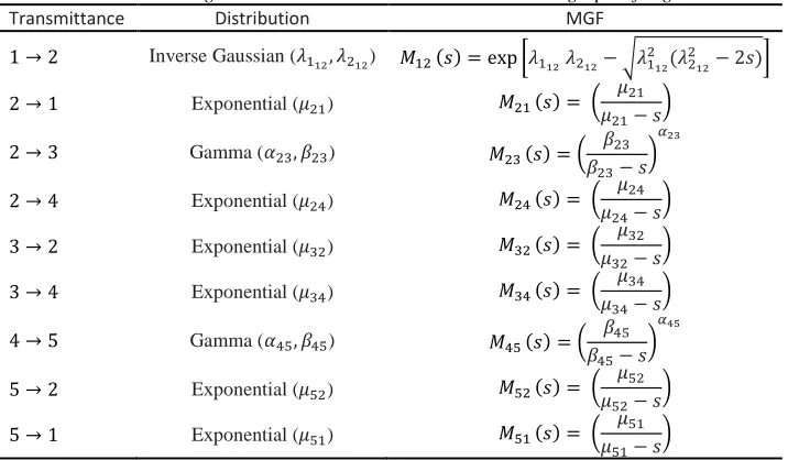
We assume a variety of waiting time distributions such as Inverse Gaussian (#, #), Gamma (%, &) and Exponential (') given in Table 2. If we had data on the real system, we would use that to select candidate distributions [4]. Parameter estimation is done by standard methods such as maximum likelihood [4] or the entire problem can be solved from the viewpoint of prediction using Bayesian methods as in Section 2.1.3.

For now, we assume the following parameter values

0.6, 0.3, 0.7, 1

, 0.5, 1 , 0.4,

0.6, 1 , # 20, # 5,

' 0.3, % 3, & 4, ' 1, '

3, ' 1, % 4, & 1, ' 0.3, '

0.5.

Table 2 Waiting Time Distributions For The Statistical Flowgraph Of Fig. 1 At End Of Text.

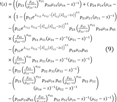
The MGF for the overall waiting time using these distributions in Eq. (8) is (from MAPLE software)

1 . . .

9

We could replace Fig. 1 with an equivalent SFGM that has only two states 2 and 4, with one connecting branch. The MGF assigned to the branch is as defined in Eq.(9).

Solving SFGMs gives us the MGF of the overall waiting time distribution of interest; however, we still have not obtained the distribution itself. The next section discusses the conversion of MGFs such as Eq.(9) to waiting time density.

2.1.2. Inversion of statistical flowgraph MGF

Note that our interest with SFGMs is to convert the resulting MGF into a density, CDF, survivor function and hazard function.

Parametric SFGMs have used MGF to represent the probability of transition between states. This has greatly limited the number of distributions available for SFGMs, since not all distributions have MGFs. Popular distributions such as the lognormal or certain Weibulls do not have MGFs and have not been used in SFGMs. By using complex Laplace Transforms (LTs) in lieu of MGFs we can use all continuous and differentiable parametric distributions in SFGMs. Complex LTs are a generalization of MGFs and characteristic functions and exist for all lifetime distributions. The Laplace Transform, as defined in statistics, is a simplification of the LT as defined in mathematics. In mathematics, the Laplace Transform, ",, is defined for all real and complex ,, while in statistics it is usually only defined for real ,. Therefore, we use the term complex LT to avoid ambiguity [3]. A complex LT for a positive random variable , defined on -0, ∞ with

, / 01and 2 0, is

", ₍₁₀₎

If the MGF has a closed analytic form, then so does

the complex LT, and finding the complex LT for the random variable is a transformation similar to finding the MGF. However, for distributions that do not have closed form MGFs we must find the complex LT or MGF by numerical integration. Examples of distributions that have closed form complex LTs are the gamma and inverse Gaussian distributions, and examples that do not are the lognormal and Weibull distributions. Using the complex LT does not change any theory we introduced in Section 2.1.1. Mason’s rule still applies; all we do is replace the MGFs with their associated complex LTs [3].

distribution in statistical flowgraph modeling. This is a big step forward for SFGMs [3].

The Euler method uses the Bromwich integral and Euler summation (and hence its name). The Bromwich contour inversion integral is [3]:

!"

#"∞

#"∞ ",,, (11)

Where 0 √1, ", is the complex LT, and the

contour is any vertical line , 4 such that "4 has no singularities on or to the right of it. With a change of variable and some manipulation, can be rewritten as

$

! -"4 / 05

∞

cos , (12) Where -,5 is the real part of a complex number. Using the trapezoidal rule with step size 9/2 and letting 4 ;/2 gives the approximation

∑ 1∞

. (13)

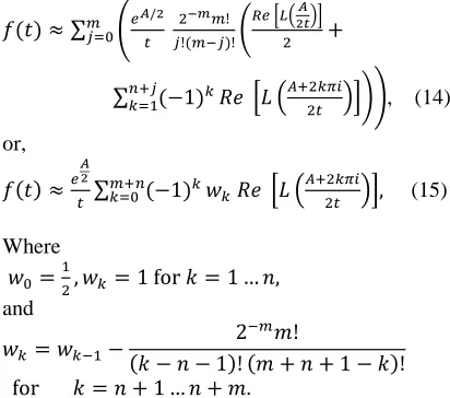
This is a nearly alternating series so Abate and Whitt [18] use Euler summation as an acceleration method. Combining these, our approximation for the density of one random variable , is

< ∑ >$ / _'!%'!%! ?($ )*+,

/

% '-

∑ 1/' .

.- " @0.!" ABC, (14)

or,

<$

∑%/.- 1.D. " @ 0.!"

A, (15)

Where

D , D. 1 for G 1 … I, and

D. D. 2

%_J!

G I 1! J / I / 1 G! for G I / 1 … I / J.

Abate and Whitt [19] recommend setting J

11, I 15, and increasing I if better accuracy is required. This approximation contains two different errors. First is the error introduced by the trapezoidal approximation, and the second by the truncated sum and Euler acceleration. Abate and Whitt [19] show how to bound the first type of error by choosing A (often they choose ; 18.4). However, the error introduced by the truncated sum

and Euler acceleration cannot be bounded, only estimated.

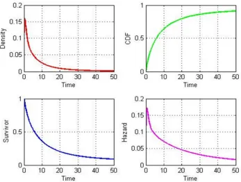
All of the distributions used in this example have closed form MGFs. Now, we use the Euler method to convert the MGF of the overall waiting time from 2 to 4 into a density. The resulting density, CDF, etc., are given in Fig. 2 (from MATLAB).

Fig. 2 Density Function, CDF, Survivor Function And Hazard Function For Example 1 At End Of Text.

SFGMs focus on modeling the observed state-to-state waiting times. This type of modeling allows us to realistically model the shape of the hazard. The shape of the hazard is increasing and decreasing at varying rates. This is typical of hazards from SFGMs since we are modeling the actual waiting times and not making assumptions about the hazards. Based on these, the purpose of plots presented in Fig. 2 is to help energy managers better understand the hazards and opportunities they face, to evaluate the options available for their control and finally to select optimal energy policies. SFGM is a useful decision support tool for survival analysis in power systems. The term decision support (DS) contains the word support, which refers to supporting people in making decisions. Thus, DS is concerned with human decision making, especially in terms of helping people improving their decision making.

Analysis from the flowgraph model gives an entire waiting time distribution as well as the system reliability (survivor) and hazard functions for any total or partial waiting time. For decision making, this immediately provides the mean, median, or any percentile of the waiting time distribution for a variety of input distributions [12].

In addition to the functions and , a common metric in power system is the mean time to failure (MTTF) which is the average time to the first failure. It can be obtained from the mean of the probability density of the time to failure :

MTTF (16)

If is the system reliability (survivor) function,

the integral in Eq. (16) becomes

MTTF which, after integrating by parts [20-22], gives

MTTF ₍₁₇₎

2.1.3. Bayesian statistical flowgraph models

Bayesian SFGMs use the same principles as frequentist SFGMs. The primary difference is that the Bayesian framework provides a posterior predictive distribution (PPD) as the final result. This is very useful since prediction is the primary focus of SFGMs. This section describes the computation of Bayesian predictive density, cumulative distribution function, survivor function, and hazard function for SFGMs using Euler method and slice sampling technique. Information about the process allows us to solve the SFGM as seen in Section 2.1.1 and Section 2.1.2. Observations on the various transitions allow us to consider parametric models for the branch waiting times of the SFGM. Our interest lies in making inferences about the unknown parameters in the model, updating our knowledge of the mechanism that generated the data, evaluating branch models, and ultimately using our data and the SFGM for prediction. Bayesian analysis formally incorporates subjective information about a problem into the analysis.

We can think about our model as the theory that drives what we can observe. For a given parameter vector P, we expect things to behave in a certain way. We use the data to give us additional information about P, but we can never know P. We know that our theory (model) is incorrect, so the question then becomes: How useful is it? What is often important is whether we can use the formulated model to make useful predictions about new observations, Q Q, … , Q, that are conditionally independent of R, the observed data, given P. In a flowgraph model, these future observations will generally be total or partial waiting times [12].

Definition (Bayes theorem). The posterior

distribution of parameter vector P given the data R is defined by

9P|R ∝ UP|R9P (18)

where UP|Ris the likelihood function and 9P

is the prior [12].

The Bayesian predictive density of a future observable Q given data R about a system with parameter vector P is

1V|R 2 _{2 65|7!55}3|565|7!55 (19)

where Q has density ₁V|P [12].

In general, we do not know ₁V|P in Eq.(19). In this case, we use W₁V|P in place of ₁V|P.

W1V|P is computed using the Euler method i.e. Eq. (14) or Eq.(15). Practically, this involves generating a random sample of P values from the posterior and performing the following computations for each P value [12]:

1. Convert the statistical flowgraph MGF,_1|5 , to a density using the Euler method for each value V of Q at which the density is desired.

2. Treat each density as a vector of values (evaluated at each value V in computation 1) indexed by P₈.

3. For each V value, average the densities

over the P values to give

X₁V|R ∑ 93|5

(20)

where W₁V|P₈ is the density derived from the

Euler method and is the number of samples. For large , this sum approximates the integral Eq.(19).

There are many methods for sampling from the posterior distribution (e.g. rejection sampling, importance sampling, Gibbs sampling, etc. [12]), and some methods are better suited than others for specific problems. A recently developed technique that lends itself to sampling from the posterior with SFGMs is a Markov Chain Monte Carlo (MCMC) method called slice sampling [12]. Slice sampling was introduced by Neal [23] and is presented in detail in [24]. The basic premise of slice sampling is that one can sample from any univariate distribution by sampling points uniformly under the graph of its density function. Multivariate slice sampling can be performed by applying a single variable slice sampling method to each variable in sequence [12]. In this study, we use Slice sampling for sampling from the posterior distribution. Our goal is to compute the Bayesian predictive density of the overall waiting time from 2 → 4 using Eq.(20). We let be this random time. Our parameter vector P is P , , , ,

, , , , , # , #, ', %, &, ', ', ', %, &, ', '.

We assume Unif0,1 priors on , , , ,

, , , and . The remaining priors

9 ', 9 ', 9%, 9& ~ Unif0,4 9', 9', 9' ~ Unif0,1 9 % , 9& ~ Unif0,2 9# ~ Unif1,5 9 # ~ Unif1,10 9' ~ Beta2,1

(21)

This computation, using M = 1000 values, gives the Bayes predictive density, CDF, survivor function, and hazard function of the waiting time of interest in Fig.3. Note that we never actually get the exact predictive density; we estimate it via the random samples.

Fig. 3. Bayes Predictive Density Function, CDF, Survivor Function And Hazard Function For Example

1 At End Of Text.

2.2.Example 2: statistical flowgraph models for power system protection: protective relay testing

The goal of protective relay testing is to maximize the availability of protection and minimize risk of relay misoperation. Having defined the necessary tests and monitoring methods for protective relays, it is now necessary to optimize the testing interval [25].

Schweitzer [25] introduced a nine-state model defined by the operating condition of the relay and the protected component. The model accounts for relay self-testing, but does not account for other monitoring means. Fig. 4 shows a ten-state model that accounts for self-testing and models routine relay verification through other simple checks. The circles represent the model states. The arrows represent the transition paths between the states.

Fig. 4 SFGM For A Protection/Component System At

End Of Text.

The model assumes that when a fault occurs while the relay is out of service, a larger portion of the power system is isolated than was actually necessary to remove the fault. The relay could be out of service because of a failure, testing, or repairs.

The probability model is divided into four quadrants representing the condition of the relay (Protection (P)) and the line (Component (C)). State 1 represents a normal operating condition where the line is energized (C UP) and the relay is operating properly (P UP). When a line fault occurs, the Component makes the transition to a down (DN) state, represented by state 2. In state 2, the line is faulted and the relay signals the circuit breaker to trip. Circuit breaker operation takes the

model system to state 6, where the line is isolated (ISO). The line is repaired and re-energized, taking the model back to state 1.

States 5, 3, 9 and 10 represent conditions where the relay is out of service and unavailable to trip if a fault occurs. In state 5, the relay is out of service for routine testing. In states 3, 9, and 10, the relay is out of service due to a relay failure. State 9 represents the relay under repair (REP). The model enters state 9 from state 1 when a relay self-test detects a failure. The model system enters state 9 from state 3 when a routine test detects a relay failure. The model enters state 9 from state 10 when a meter check detects a failure.

The model enters state 3 from state 1 when a relay failure occurs that is not detected by the relay self-test function and could not be detected by meter checks.

A failure not detected by either self-tests or meter tests are only detected by routine testing or by observing a misoperation. The model enters state 4 if a fault occurs while the relay is out of service, or if a common-cause failure of the relay and power system occurs. If a fault occurs while the relay is out of service, remote backup protection operates to isolate the fault. When the remote protection operates, a larger portion of the power system is taken out of service than would have been if the failed relay had operated properly. This is represented in state 4 and state 8 by the isolation of C and X, where X is the additional equipment removed from service by the backup relay trip operation.

Consider the SFGM in Fig. 4. Quantity of interest includes predicting the distribution of the total waiting time from state 1 to state 4. There are eight paths from 1 to 4 (e.g.1 → 3 → 9 → 4). Also, there are nineteen first-order loops (e.g.1 → 2 → 6 →

7 → 9 → 1) and six second-order loops (e.g.

1 → 3 → 9 → 1 with 6 → 7 → 6) . In this analysis, the waiting time distribution for transition from any state to any state is assumed to be Exponential ('). Applying Mason’s rule we find the MGF of the overall waiting time distribution from state 1 to state 4. Finally, we transform this MGF into a density, CDF, etc. They are shown in Fig. 5.

Fig. 5 Density Function, CDF, Survivor Function And Hazard Function For Example 2.

Fig. 6 Bayes Predictive Density Function, CDF, Survivor Function And Hazard Function For Example 2 At End Of

Text

3. CONCLUSION

The aim of survival analysis is to estimate the distribution of the time it takes for events to occur. This paper proposed statistical flowgraph models (SFGMs) as a new approach to do survival analysis in power systems. This decision support tool (using the semi-Markov assumption) provides a way for analyzing time-to-event data and constructing corresponding Bayesian predictive distributions. SFGMs allow data analysis for semi-Markov processes using non-exponential waiting times. They can be applied without becoming intimately familiar with the mathematical theory of stochastic processes. While the increase number of states improves the accuracy of modeling power systems, it also brings the problem of whether proposed multistate models can be compatible with practical studies. Therefore, it is necessary to find a method to reduce multistate models into an equivalent binary-state model, to ensure proposed models are practical. SFGMs provide a systematic way that can be used to reduce complex power systems models. The approach advances the state of the art in power system survival analysis. It also lays a general foundation for effective and systematic power system management.

SFGMs model the observable waiting times rather than the hazards and as such, they do not directly make any assumptions about the shape of the hazard. For decision making, this immediately provides the mean, median, or any percentile of the waiting time distribution for a variety of input distributions [12].

ACKNOWLEDGMENTS

I am thankful to Department of Electrical and Computer Engineering, Behbahan Branch, Islamic Azad University, Behbahan, Iran for their support and collaboration on the design of the presented exercises and sharing their pandemic preparedness plans with me.

REFRENCES:

[1] D. G. Kleinbaum, M. Klein, Survival Analysis: A Self-Learning Text, second ed., Springer-Verlag, New York, 2005.

[2] Leonel de Magalhães Carvalho, Using evolutionary swarms (epso) in power system reliability indices calculation, Master thesis, University of Porto, Porto, Portugal, 2008. [3] R.L. Warr, Generalizations of the statistical

flowgraph model framework, PhD thesis, University of New Mexico, Albuquerque, NM, 2010.

[4] A.V. Huzurbazar, Flowgraph models: a Bayesian case study in construction engineering, J. Stat. Plann. Infer. 129 (2005) 181–193.

[5] S.J. Mason, Feedback theory: some properties of signal flow graphs, Proc. Inst. Radio Eng. 41(1953) 1144–1156.

[6] R.W. Butler, A.V. Huzurbazar, Stochastic network models for survival analysis, J. Am. Stat. Assoc. 92 (1997) 246–257.

[7] A.V. Huzurbazar, Flowgraph models for generalized phase type distributions with non-exponential waiting times, Scand. J. Stat. 26 (1999) 145–157.

[8] A.V. Huzurbazar, Modeling and analysis of engineering systems data using flowgraph models, Technometrics, 42 (2000) 300–306. [9] R.W. Butler, A.V. Huzurbazar, Bayesian

prediction of waiting times in stochastic models, Can. J. Stat. 28 (2000) 311–325. [10]C. L. Yau, A.V. Huzurbazar, Analysis of

censored and incomplete survival data using flowgraph models, Stat. Med. 21 (2002) 3727– 3743.

[11]A.V. Huzurbazar, Multistate models, flowgraph models, and semi-Markov Processes, Comm. Stat. Theor. Meth. 33 (2004) 457–474.

[12]A.V. Huzurbazar, Flowgraph models for multistate time-to-event data, John Wiley & Sons, New York, 2005.

[13]A.V. Huzurbazar, Modeling time-to-event data using flowgraph models, in: N. Balakrishnan (ed.). Advances on methodological and applied aspects of probability and statistics, Taylor and Francis, New York, 2000, pp. 561–571. [14]A.V. Huzurbazar, B.J. Williams, Flowgraph

Models for complex multistate system reliability, in: A.G. Wilson, N. Limnios, S.A. Keller-McNulty, Y.M. Armijo (eds.), Modern statistical and mathematical methods in reliability, Singapore: World Scientific, 2005, pp. 247–262.

23: advances in survival analysis, Elsevier, Amsterdam, 2004, pp. 729–746.

[16]P. K. Andersen, N. Keiding, Multi-state models for event history analysis, Stat. Methods Med. Res. 11 (2002) 91–115. [17]P. Kundur, Power system stability and control,

McGraw-Hill, 1994.

[18]J. Abate, W. Whitt, The Fourier-series method for inverting transforms of probability distributions, Queueing Syst. 10 (1992) 5–88. [19]J. Abate, W. Whitt, Numerical inversion of

Laplace transforms of probability distributions, Informs J. Comput. 7 (1995) 36–43.

[20]D.L. Grosh, A Primer of Reliability Theory, John Wiley & Sons, Inc., New York, 1989. [21]R. Billinton, R. N. Allan, Reliability

Evaluation of Engineering Systems: Concepts and Techniques, Plenum Press, first ed., New York, 1983.

[22]J. Endrenyi, Reliability modeling in electric power systems, John Wiley & Sons, New York, 1978.

[23]R. Neal, Markov chain Monte Carlo methods based on “slicing” the density function, Technical Report 9722, Department of Statistics, University of Toronto, Ontario, Canada, 1997.

[24]R. Neal, Slice sampling, Ann. Stat. 31 (2003) 705–767.

TABLES

Table 1 Paths And Loops For Solving The Statistical Flowgraph Of Fig. 1

Path Transmittance

Path 1: 2 → 4

Path 2: 2 → 3 → 4

1

-order loops

1 → 2 → 1

2 → 3 → 2

2 → 4 → 5 → 2

2 → 3 → 4 → 5 → 2

1 → 2 → 4 → 5 → 1

1 → 2 → 3 → 4 → 5 → 1

Table 2 Waiting Time Distributions For The Statistical Flowgraph Of Fig. 1

Transmittance Distribution MGF

1 → 2 Inverse Gaussian (_భమ, _భమ) exp _{భమ భమ భమ}

_భమ

2

2 → 1 Exponential ()

2 → 3 Gamma (, )

మయ

2 → 4 Exponential ()

3 → 2 Exponential ()

3 → 4 Exponential ()

4 → 5 Gamma (, )

రఱ

5 → 2 Exponential ()

5 → 1 Exponential ()

FIGURES

1

Normal

5

Restorative

2

Alert

4

In extremis

3

Emergency

p

M

(s)

p

M

(s)

p

M

(s)

p

M

(s)

p

M

(s)

p

M

(s)

p

M

(s)

p

M

(s)

p

M

(s)

Fig. 2. Density Function, CDF, Survivor Function And Hazard Function For Example 1.

2

C DN P UP

6

C ISO P UP

7

C ISO P DN

8

C+X ISO P DN

4

C+X DN P DN

1

C UP P UP

10

C UP P DN

5

C UP P INS

3

C UP P DN

9

C UP P REP

p26M26(s)

p67M67(s)

p87M87(s)

p48M48(s) p12M12(s)

p110M110(s)

p104M104(s) p54M54(s) p34M34(s) p13M13(s)

p109M109(s)

p39M39(s)

p19M19(s) p91M91(s)

p94M94(s) p79M79(s)

p76M76(s) p61M61(s)

p14M14(s) p51M51(s)

p15M15(s)

PROTECTION UP COMPONENT

UP

COMPONENT DOWN

PROTECTION DOWN

Fig. 5. Density Function, CDF, Survivor Function And Hazard Function For Example 2.