Development of a Consignment Inventory Model in a Two- echelon Supply Chain with Backorder

(1)

International Journal of Emerging Technology and Advanced Engineering

Website: www.ijetae.com (ISSN 2250-2459,ISO 9001:2008 Certified Journal, Volume 3, Issue 1, January 2013)

90

Development of a Consignment Inventory Model in a

Two-echelon Supply Chain with Backorder

Zohreh Molamohamadi

1

, Napsiah Ismail

2

, Zulkiflle Leman

3

,

Norzima Zulkifli

4 1,2,3,4

University Putra Malaysia, Faculty of Engineering, Department of Mechanical and Manufacturing Engineering

Abstract— This paper considers a two-level supply chain consisting of a manufacturer and two buyers. The manufacturer produces one type of products at a finite rate and replenishes them to the buyers. Each buyer’s demand is sensitive to his selling price and the backorder is allowed at the buyers. Moreover, it is assumed that the buyers delay paying for goods to the manufacturer and two types of delay in payment are considered; delay paying for the purchased items till they are used or sold to the end customers, and delay paying till the next replenishment order. The main aim of this research is formulating the manufacturer and the buyers’ problems in terms of integer-ratio policy and discounted cash flow under these two types of delay in payment.

Keywords— Consignment inventory, delay in payment, discounted cash flow, trade credit, two-echelon supply chain.

I. INTRODUCTION

Consignment inventory (CI) is an agreement between a supplier and his customer in which invoicing is delayed until the time agreed upon. In such a contract, the ownership will not be transferred from the supplier to the customer immediately when the products are shipped; There are four types of CI based on how long the goods are on consignment ([1],[2]): 1) until the goods are used by the customer 2) until they are used during a predefined period, 3) until a predefined period, and 4) until the next order is placed.

CI is beneficial to the customer especially when there is uncertainty in the final demand. It also benefits the supplier by creating new sales channels when there are new, unproven, or expensive products that the customer hesitates to buy.

Most of the studies conducted in consignment inventory have considered the second and third types of delay in payment. These types have been referred to as trade credit in the literature and the delayed period is known as credit period.

This paper aims at considering a manufacturer who supplies an item to two different buyers. The production rate is finite and the demand that the buyers are faced is a decreasing function of their selling prices.

Shortages may occur at the retailers and they are allowed to delay paying to the supplier until they sell the item to the customer (CI type 1). The objective here is to formulate the net profit of this two-echelon supply chain in terms of integer-ratio policies and considering the time value of money.

The rest of this paper is organized as follows: Section II reviews the CI related literature. In section III, assumptions and notations for stating the problem are introduced. Section IV discusses the applied inventory policy. The problems are formulated in section V and the conclusion is presented in section VI.

II. CONSIGNMENT INVENTORY:LITERATURE REVIEW

This section classifies some of the conducted researches in consignment inventory based on the delay in payment type.

A. Pay as sold

(2)

International Journal of Emerging Technology and Advanced Engineering

91

B. Pay as sold during a predefined period

In this type of CI, a predefined period, so-called credit period, is considered and the payment for the goods is settled when they are sold. At the end of the credit period, the customer can decide to either pay for the unsold inventory or send them back to the vendor.

Reference [7] analyzed the optimal inventory policy by employing discounted cash flows (DCF) approach under the trade credit terms. Reference [8] obtained the optimal order quantity of deteriorating items to extend [7]. Reference [9] generalized [8] by applying order quantity dependent trade credit. Reference [10] discussed the influence of DCF approach and trade credit on the optimum cycle time and order quantity to extend [7]. They assumed that delay in payment is allowed only if the order quantity is greater than a predefined period. This type of contract is known as order quantity-dependent trade credit. By using numerical examples, [11] showed that the approximate optimum solutions obtained by [8] are not always appropriate. Thus, they proposed an algorithm to find the optimal cycle time.

C. Pay after a predefined period

This contract, called trade credit in the literature, allows the customer to settle the account at the end of a certain fixed period. During this credit period the retailer can sell the items to accumulate revenues and earn interest, but after this period he will be charged for the items in stock. Trade credit has been widely discussed during the past decades.

Reference [12] determines the optimal order quantity under trade credit by proposing a mathematical model. Reference [7], and Reference [8] (also mentioned in part B) considered fixed credit period as another case in their studies. Reference [13] developed [12] ’s model to the case of deterioration. Reference [14] encompassed shortage in the previous model that is completely backlogged. Reference [15] found a theorem through alternative approach and simplified the solution procedure described in [12]. Reference [16] overcome [13] by developing a new solution procedure. Reference [17] further generalized [13] with allowing for partial shortages. Reference [18] extended [12] ’s EOQ model to an EPQ model in which the replenishment rate is finite. Reference [19] generalized [12]’s model by considering a two-level trade credit. Reference [20] compared the order-size-dependent trade credit with [12]’s proposed model. Reference [21] assumed that carrying cost rate, interest paid rate and interest earned rate in the proposed model by [14] may have fuzzy values.

Reference [22] developed [19] by assuming limited storage space for the retailer. Reference [23] proposed a model for deteriorating items and limited storage capacity to modify [19]’s model. By considering credit-linked demand rate, [24] established a trade credit model in which the retailer provides the customers with shorter credit period than what he is provided by the supplier. Reference [25] further incorporated [18] and [19] to analyze the retailer’s replenishment decision in an EPQ framework and two levels of trade credit. Reference [26] developed [19] by presenting an EPQ model for exponentially deteriorating items. Reference [27] followed [12] to develop a new model with permitted shortages. Reference [28] complemented the shortcoming of [25] and further developed it by considering that the retailer’s credit period may also be smaller than the customer’s credit period. Reference [29] proposed an EPQ model under two-level trade credit with defective items when delay in payment depends on the quantity ordered. Reference [30] formulated retailer’s EOQ model with deteriorating items and fluctuating demand under two-level trade credit. Reference [31] considered inflation, deterioration and time value of money in a general finite horizon trade credit inventory model with time-dependent demand and deterioration rate. Reference [32] presented a two-level trade credit model for defective items in an EPQ framework.

Reference [33] extended [24] by assuming that the retailer credit period might be smaller or greater than the supplier credit period and considering the price and credit linked demand rate. Reference [34] considered a multi-item supply chain under delay in payment and weight freight cost discounts to formulate the optimization models from individual and channel perspectives. Reference [35] generalized [18], [19] and [22] and formulated an EPQ model by assuming two level trade credit, limited storage capacity and different selling and purchasing prices. Under permissible delay in payment, Yu [36] examined an integrated inventory system for deteriorating items with price-sensitive demand and completely backordered shortage and concluded that supplier-buyer collaboration would result in extra profit gain. Yang and Chang [37] developed an inventory model by considering two warehouses with different deterioration rates and partially backlogged shortages to find the optimal replenishment policy under DCF approach.

D. Pay after next consignment order

(3)

International Journal of Emerging Technology and Advanced Engineering

92

Reference [38] represented a model under continuous review inventory in which the retailer can choose between paying at the time of receipt or delaying till the next replenishment order and being charged simple interest. Besides considering the real use as the time of payment, which was mentioned in A, [4] also formulated a model for the case in which the retailers delay paying to the warehouse for one cycle time.

Generally, this type of CI has not been specifically discussed in the literature, but it is considered as a special case in the aforementioned studies in sections 3.2 and 3.3 where the credit period is less/greater than or equal to the cycle time.

Reviewing the literature clarifies the existing gap in two types of delay in payment (pay as sold and pay after next replenishment order). For contributing to the existing literature and covering a small area of this gap, we focus here on modeling the consignment inventory in a supply chain under two types of delay in payment; where the two retailers delay paying to the manufacturer till the time of selling (first type of consignment contract) and order to order consignment (fourth type).

III. ASSUMPTIONS AND NOTATIONS

To model the problem, the following notations are applied:

i: index of the retailers, i1, 2;

( )

i pi

D : demand of the retailer i per unit time which is a function of p_i;

pi

e : price elasticity of retailer i’s demand rate;

i

k : a constant in demand function of retailer i, which represents his market scale;

m

v : procurement price of the product for manufacturer ($/unit);

m

h : holding cost of the manufacturer ($/unit/time);

r

p : constant production rate of the manufacturer;

p

S : production setup cost at the manufacturer;

bi

A : fixed replenishment cost per order for retailer i

($/order);

i

 : direct transportation cost for shipping one unit product from the manufacturer to retaileri ($/unit);

si

h : physical storage cost of the retailerifor one unit in stock ($/unit);

i

B : backorder cost of retaileri($/unit/time);

r: interest rate;

i

b : fraction of backlogging time in a cycle of retaileri;

v

t : the time interval between two consecutive setups at the manufacturer;

i

t : replenishment interval at retaileri; p

c : wholesale price of the product set by the manufacturer ($/unit); and

i

p : retail price of retaileri($/unit).

Among these symbols, b_i, t_v, t_i, _c_p, andp_ican be considered as decision variables.

The following assumptions will also be considered in the formulation of the model:

(1) One manufacturer produces and transfers one type of product to his two independent retailers who serve their own markets. Demand of each retailer is price-dependent and described by Cobb-Douglas demand function as (1):

( ) pi, 1, 2

i pi kip e i

D  _i  (1) (2) Integer-ratio policy is used to formulate the one manufacturer and two-buyer consignment inventory system.

(3) The first and last types of delay in payment are considered and the inventory models are formulated. (4) Because the manufacturer’s production capacity is

limited, the total demand of the two buyers must be less than the production rate.

(5) Shortage is allowed at the retailers’ sides. (6) Lead time is negligible and not considered.

(7) DCF approach is applied here to consider the time value of the money and the interest rate compounds continuously.

IV. INVENTORY POLICY

The model in this paper is formulated in terms of integer-ratio policy and is confined to the integer-ratio policies that t2/t1is a positive integer. This means that when the retailer 2 places an order, so does the retailer 1. Therefore, there will be some points in time when the manufacturer supplies to both retailers simultaneously, and others that only retailer 1 is supplied. Accordingly, the manufacturer should start the production sooner when he has to supply to both buyers, compared with the case that only retailer 1 should be supplied.

(4)

International Journal of Emerging Technology and Advanced Engineering

93

[image:4.612.52.292.213.392.2]

Yet, considering only retailer 1 and supposing that the manufacturer produces first the units to be sent to retailer 2, then the time interval between two consecutive setups, between A and B (denoted byt₀) in Figure 1 will be constant.

Figure 1. Inventory fluctuations at the manufacturer and at the buyers

So, t0is the time interval between two consecutive setups only for the retailer withtitv (i1 here). Then

the time interval between two consecutive setups for the retailer with titv(i2 in this example) can be easily

obtained from t₀. For integer-ratio policy with respect tot0, we assume that either ti/t0or t0/ti(i1, 2) is a

positive integer.

V. MODEL FORMULATION

The model formulation of the net profit for the manufacturer and retailers under two types of delay in payment (the first and the last types) are represented in this section.

Because the inventory models of the retailers follow an EOQ model, obtaining their average inventories is not difficult and can be formulated as follows.

A. Retailers’ net profit models

Pay when the items are used/ sold: Each buyer’s net profit

model for the first type of delay in payment is formulated in (2).

The model consists of retailer i’s revenue, the product

procurement cost with considering the DCF approach (including the procurement cost for the time of backorder and for the time with on hand inventory), inventory holding cost, backorder cost, replenishment cost and transportation cost, respectively.

1

2 2 (1 )

0

2 2 (

(1 ) )

2

pi pi

pi

i i pi

pi

i i i p i i i

i i

rt

p i si

i

i i i bi

i i i

i i

e e

p p

p

NP k _i c k _i b t

e

p b

k i i t

b t _{c k} _p e _e _dt _h

i

t e

p

k i b t _B A _k _p e

i

t t

 



  _



  



 



  

(2)

where

(1 ) ₍₁ ₎

0

1

(1 )

i i pi rt pi r _i _i

p i p i

b t _p e _dt _p e _t _b

c k _i e c k _i e

r

  _ _  _ _ _

 (3)

1) Pay at the next replenishment: the only difference

between this type of delay in payment and the previous mentioned type is in the procurement cost. Considering order to order consignment inventory, the retailers’ net profit function would be changed to (4).

2

2 2

2 2 (1 ) 2

2

pi pi i

pi

rt

i i i p i

i i

si i

i i i bi

i i i

i i

e e

p p

p

NP k _i c k _i e

e

p b

k i i t

h t

e p

k i b t _B A _k _p e

i

t t

  _



 



 

  

(4)

B. Manufacturer’s net profit model

From the manufacturer’s side, since his average inventory differs based on whether t1 t2 t0or

1 0 2

t  t t , computing the average inventory of the manufacturer is more complex and we will explain it in the following subsections.

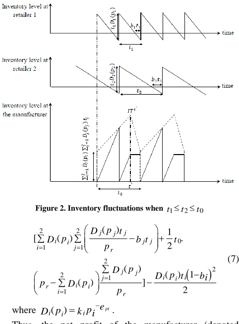
1) Pay when the items are used/ sold: Figure 2 is

illustrated here for computing the manufacturer’s inventory holding cost whent1 t2 t0by supposing thatt¢is the point in time when the inventory of the system reaches its maximum (ITt

¢

).

We can see from Figure 2 that

2

1

0

e pi i i

r p k _i

t _p t

 



(5)

International Journal of Emerging Technology and Advanced Engineering

94 2 2 1 1 2 2 ₁ 0 1 pi pi pi pi i j

i j j

i j _r

i j i r i _r e p

k _i t

e

t _k p _{b t}

IT i p e p k _i e p p

t k _i

p                        _   _   ¢ (6)

[image:5.612.48.571.97.629.2]

Thus, the average inventory at the manufacturer will be obtained by subtracting the average inventory at the buyers from the total average inventory as it is shown in (7),

Figure 2. Inventory fluctuations when t₁ t₂ t₀





2 2 0 1 1 2 2 2 ₁ 1

( ) ₁

[ ( ) .

2

( )

( ) 1

( ) ]

2

j j j

i i j j

i j _r

j j i i j i i r i i _r p t D

p b t t

D

p

p D

p t b

D i

p D p

p           _ _    _  _  _      (7)

where ( ) pi

i pi kip e

D  _i .

Thus, the net profit of the manufacturer (denoted byNP_m₁) including the revenue, procurement cost, inventory holding cost and setup cost, when t1 t2 t0, is formulated in (8).









2 1 1 2 2 (1 ) 1 1 2 2 0 1 1 2 2 2 ₁ 1 0 1 1 1 [ ( ) 2 1 . ] 2 pi i

pi _i _i pi

pj pi pj pi pi r

ma p i i i

i

p i m i i

i

j j

m i j j

i j r

j i i j p i r i r e t p

NP c k _i b t e

e rt b e

p p

c k _i e v k _i

r

e p

k j t

e p

h k _i b t t

p

e p

k j _p e

k i t bi S

e p

p k i

p t     _ _                                  

(8)

So, the model of the manufacturer in this case would be

1 max . pi ma i r NP e p

st k _i  p

(9)

The case in whicht1 t0 t2, is depicted in Figure 3. Two inventory types are considered for the manufacturer in Figure 3, one of which is for satisfying the retailer 1’s demand and the other for meeting the needs of retailer 2.

Figure 3. Inventory fluctuations when t₁ t₀ t₂

Based on this figure, _t¢and _ITt¢can be formulated in (10) and (11) respectively.

1( 1)

0

r p D

t¢ _p t (10)





1 1 1 1 0

1 1 1 1 1 1

( ) ( )

( ) ( ) _r ( )

r r

p p t

D D

t p t b p p

IT D D

p p

   

¢

[image:5.612.47.288.263.590.2] [image:5.612.325.563.373.606.2]

(6)

International Journal of Emerging Technology and Advanced Engineering

95

So, the average inventory at the manufacturer for retailer 1 can be calculated by deducting the average inventory of the retailer 1 from the total average inventory as follows;









1 1 1 1 0

1 1 1 1 1 1

2 1 1 1

( ) ( )

( ) 1 ₁

2

r

r r

p p t

D D

p t b p p

D D

p p

p t b

D              (12)

In this case the manufacturer only keeps inventory for retailer 2 during the production time, not after the shipment. So, (13) represents the manufacturer’s average inventory for retailer 2.

2

1 1 1

1

( ) ( )

2 2

2 ( )

i i i i

r p t p t

D D p D p    (13)

Assumingt₁ t₀ t₂, the net profit of the manufacturer (NPmb1) is shown in (14) when the payment is settled at the time of selling or consuming the product.













1 1 1 1 1 2 ₁ 1 1 1 2 1 2 1 2 ₁

1 1 1

1 2 1 1 1 0 1 2 0

1 (1 )

1 [ ₁ 1 ₁ 1 1 .

1 ₂ ₂

1

] 2 2

pi

pi _i _i

p

pi p

p p

p

epi ep

i i i p r mb p i r r

p i i i i

i

m i m

i _r r r p NP e p

c k _i

e _t _t

p

c k _i b t e e b

r e p k e e p p

v k _i h k t b

p

e

e _p

p k t b

k t e p p k p p p

k _i t k t _S

e p k p      _ _                                 _ _         t (14)

The components of (14) are manufacturer’s revenue, procurement cost, inventory holding cost, and setup cost, respectively.

Considering (14) as the net profit of the manufacturer whent₁ t₀ t₂, the model of the manufacturer is represented in (15).

1 max . pi mb i r NP e p

st k _i  p

(15)

2) Pay at the next replenishment: The net profit functions

of the manufacturer when the retailers pay for purchased items at the time of proceeding order are formulated in (16) and (17) for the time t₁ t₂ t₀ and t₁ t₀ t₂

respectively.





2 2 2 1 1 2 2 0 1 1 2 2 2 ₁ 1 0 1 [ ( ) 2 1 . ] 2

pi i pi

pj pi pj pi pi rt

ma p i m i i

i

j j

m i j j

i j _r

j i i j p i r i _r e e p p

NP c k i e v k i

e p

k j t

e p

h k _i b t t

p

e p

k j _k _p e _t _b _S

i i

e p

p k _i

p t  _                      _          (16)









1 1 1 1 1 2 1 1 1 1 2

2 2 2

2

1 1 1

1

1 1 1

2 1 1 1 0 1 2 0 1 [ ₁ 1 ₁ 1 1 . 1 2 2 1 ] 2 2

pi i pi

p p

p

epi ep

i i

i p

r

rt

mb p i m i

i i i

m r r r p e e p p

NP c k i e v k i

e p k e p

h k t b

p

e

e _p

p k t b

k t e p p k p p p

k _i t k t _S

e p k p _t     _                                  (17)

So, the models of the manufacturer for order to order consignment when t1 t2 t0 and t1 t0 t2, are shown in (18) and (19) respectively.

2 max . pi ma i r NP e p

st k _i  p

(18) 2 max . pi mb i r NP e p

st k _i  p

(19)

VI. CONCLUSION

(7)

International Journal of Emerging Technology and Advanced Engineering

96

REFERENCES

[1 ] Piasecki, D., ―Consignment inventory: What is it and when does it make sense to use it?,‖ Inventory Operations Consulting LLC, 2004. [2 ] Molamohamadi, Z., Rezaeiahari, M., & Jafari, A., ―Consignment

inventory: a literature review and critique,‖ in presented at the International Conference of Operations and Supply Chain Management, 2009.

[3 ] Gümüş, M., Jewkes, E. M., & Bookbinder, J. H., 2008. ―Impact of consignment inventory and vendor-managed inventory for a two-party supply chain,‖ International Journal of Production Economics, vol. 113, no. 2, pp. 502–517.

[4 ] Sharifyazdi, M., Jafari, A., Molamohamadi, Z., Rezaeiahari, M., & Arshizadeh, R., ―Particle Swarm Optimization Approach in a Consignment Inventory System,‖ in Numerical Analysis and Applied Mathematics: International Conference on Numerical Analysis and Applied Mathematics, 2009, pp. 240–243.

[5 ] Ru, J., & Wang, Y., 2010. ―Consignment contracting: Who should control inventory in the supply chain?,‖ European Journal of Operational Research, vol. 201, no. 3, pp. 760–769.

[6 ] Adida, E., & Ratisoontorn, N., 2011. ―Consignment contracts with retail competition,‖ European Journal of Operational Research, vol. 215, no. 1, pp. 136–148.

[7 ] Chung, K. H., 1989. ―Inventory control and trade credit revisited,‖ Journal of the Operational Research Society, vol. 40, no. 5, pp. 495– 498.

[8 ] Jaggi, C. K., & Aggarwal, S. P., 1994. ―Credit financing in economic ordering policies of deteriorating items,‖ International Journal of Production Economics, vol. 34, no. 2, pp. 151–155.

[9 ] Chung, K. J., & Liao, J. J., 2006. ―The optimal ordering policy in a DCF analysis for deteriorating items when trade credit depends on the order quantity,‖ International Journal of Production Economics, vol. 100, no. 1, pp. 116–130.

[10 ]Chung, K. J., & Liao, J.-J., 2009. ―The optimal ordering policy of the EOQ model under trade credit depending on the ordering quantity from the DCF approach,‖ European Journal of Operational Research, vol. 196, no. 2, pp. 563–568.

[11 ]Chung, K. J., & Lin, S. Der, 2011. ―The inventory model for trade credit in economic ordering policies of deteriorating items in a supply chain system,‖ Applied Mathematical Modelling, vol. 35, no. 6, pp. 3111–3115.

[12 ]Goyal, S. K., 1985. ―Economic Order Quantity Under Conditions of Permissible Delay in Payments,‖ Journal of the Operational Research Society, vol. 36, no. 4, pp. 335–338.

[13 ]Aggarwal, S. P., & Jaggi, C. K., 1995. ―Ordering Policies of Deteriorating Items Under Permissible Delay in Payments,‖ Journal of the Operational Research Society, vol. 46, no. 5, pp. 658–662. [14 ]Jamal, A. M. ., Sarker, B., & Wang, S., 1997. ―An ordering policy

for deteriorating items with allowable shortage and permissible delay in payment,‖ Journal of the Operational Research Society, vol. 48, no. 8, pp. 826–833.

[15 ]Chung, K. J., 1998. ―A theorem on the determination of economic order quantity under conditions of permissible delay in payments,‖ Computers and Operations Research, vol. 25, no. I, pp. 49–52. [16 ]Chu, P., Chung, K.-J., & Lan, S.-P., 1998. ―Economic order quantity

of deteriorating items under permissible delay in payments,‖ Computers and Operations Research, vol. 25, no. 10, pp. 817–824.

[17 ]Chang, H., & Dye, C., 2001. ―An inventory model for deteriorating items with partial backlogging and permissible delay in payments An inventory model for deteriorating items with partial backlogging,‖ International Journal of Systems Science, vol. 32, no. 3, pp. 345–352.

[18 ]Chung, K. J., & Huang, Y. F., 2003. ―The optimal cycle time for EPQ inventory model under permissible delay in payments,‖ International Journal of Production Economics, vol. 84, no. 3, pp. 307–318.

[19 ]Huang, Y.-F., 2003. ―Optimal retailer’s ordering policies in the EOQ model under trade credit financing,‖ Journal of the Operational Research Society, vol. 54, no. 9, pp. 1011–1015.

[20 ]Chung, K. J., Goyal, S. K., & Huang, Y. F., 2005. ―The optimal inventory policies under permissible delay in payments depending on the ordering quantity,‖ International Journal of Production Economics, vol. 95, no. 2, pp. 203–213.

[21 ]Chen, L. H., & Ouyang, L. Y., 2006. ―Fuzzy inventory model for deteriorating items with permissible delay in payment,‖ Applied Mathematics and Computation, vol. 182, no. 1, pp. 711–726. [22 ]Huang, Y.-F., 2006. ―An inventory model under two levels of trade

credit and limited storage space derived without derivatives,‖ Applied Mathematical Modelling, vol. 30, no. 5, pp. 418–436. [23 ]Chung, K. J., & Huang, T. S., 2007. ―The optimal retailer’s ordering

policies for deteriorating items with limited storage capacity under trade credit financing,‖ International Journal of Production Economics, vol. 106, no. 1, pp. 127–145.

[24 ]Su, C.-H., Ouyang, L.-Y., Ho, C.-H., & Chang, C.-T., 2007. ―Retailer’s inventory policy and supplier’s delivery policy under two-level trade credit strategy,‖ Asia-Pacific Journal of Operational Research, vol. 24, no. 5, pp. 613–630.

[25 ]Huang, Y.-F., 2007. ―Optimal retailer’s replenishment decisions in the EPQ model under two levels of trade credit policy,‖ European Journal of Operational Research, vol. 176, no. 3, pp. 1577–1591. [26 ]Liao, J.-J., 2008. ―An EOQ model with noninstantaneous receipt and

exponentially deteriorating items under two-level trade credit,‖ International Journal of Production Economics, vol. 113, no. 2, pp. 852–861.

[27 ]Chung, K. J., & Huang, C. K., 2009. ―An ordering policy with allowable shortage and permissible delay in payments,‖ Applied Mathematical Modelling, vol. 33, no. 5, pp. 2518–2525.

[28 ]Teng, J., & Chang, C.-T., 2009. ―Optimal manufacturer’s replenishment policies in the EPQ model under two levels of trade credit policy,‖ European Journal of Operational Research, vol. 195, no. 2, pp. 358–363.

[29 ]Kreng, V. B., & Tan, S.-J., 2010. ―The optimal replenishment decisions under two levels of trade credit policy depending on the order quantity,‖ Expert Systems with Applications, vol. 37, no. 7, pp. 5514–5522.

[30 ]Dye, C.-Y., & Ouyang, L.-Y., 2011. ―A particle swarm optimization for solving joint pricing and lot-sizing problem with fluctuating demand and trade credit financing,‖ Computers & Industrial Engineering, vol. 60, no. 1, pp. 127–137.

(8)

International Journal of Emerging Technology and Advanced Engineering

97 [32 ]Kreng, V. B., & Tan, S.-J., 2011. ―Optimal replenishment decision

in an EPQ model with defective items under supply chain trade credit policy,‖ Expert Systems with Applications, vol. 38, no. 8, pp. 9888–9899.

[33 ] Ho, C.-H., 2011. ―The optimal integrated inventory policy with price-and-credit-linked demand under two-level trade credit,‖ Computers & Industrial Engineering, vol. 60, no. 1, pp. 117–126. [34 ]Tsao, Y.-C., & Sheen, G.-J., 2012. ―A multi-item supply chain with

credit periods and weight freight cost discounts,‖ International Journal of Production Economics, vol. 135, no. 1, pp. 106–115. [35 ]Chung, K. J., 2012. ―The EPQ model under conditions of two levels

of trade credit and limited storage capacity in supply chain management,‖ International Journal of Systems Science, pp. 1–17.

[36 ]Yu, J. C. P., ―A collaborative strategy for deteriorating inventory system with imperfect items and supplier credits,‖ International Journal of Production Economics, .

[37 ]Yang, H.-L., & Chang, C.-T., ―A two-warehouse partial backlogging inventory model for deteriorating items with permissible delay in payment under inflation,‖ Applied Mathematical Modelling, . [38 ]Salameh, M. K., Abboud, N. E., El-Kassar, a. N., & Ghattas, R. E.,

2003. ―Continuous review inventory model with delay in payments,‖ International Journal of Production Economics, vol. 85, no. 1, pp. 91–95.