* Studies included within the EDUCATIONAL classification are, in most coses, derived from the brood spectrum of scientific dnd engineering computer applications. Their presentation is oriented toward classroom or laboratory use, and they deal with problems appropriate for chemical, electronics, bio-medical, etc., courses. For the convenience of users in specific industrial fields, however, all EDUCATIONAL studies are cross-referenced in the Applications Library Index under the industrial activity(ies) with which they are most closely associated.
SOLUTION OF MATHIE US' EQUATION ON THE ANALOG COMPUTER
Many physical systems can be described analytically in terms of the functions of mathematical physics
such as Bessel, Mathieu, and Hypergeometric func-tions. However, an analytical solution of this type
is of little value to the investigator unless it can be
transformed into usable, numerical results. This transformation often is time consuming and
ex-pensive, especially for multiple or trial-and-error
computations. For this reason, many of these
equations, whose practical solutions are prohibi-tive, are solved on a general purpose analog com-puter. The analog computer, which may be pro-grammed with ease, produces continuous, graphical results and allows the analyst to vary parameters in a few seconds for multiple computations, thereby reducing the time and expense required to obtain usable numerical results.
Since the equations of mathematical physics de-scribe the behavior of a great many physical sys-tems, and since the analog computer is a valuable tool in obtaining their solution, it would be ad-vantageous to present the analog computer solu-tion to as many of these equasolu-tions as possible. Obviously, this is impractical; however, a typical example can be illustrated. The illustration se-lected is Mathieus' equation whose solution is unique in that it can be stable or unstable, periodic or non-periodic. Mathieus' equation is a practical illustration, also, since it describes the behavior of
1) wave guides
2) moving coil loud-speakers
3) vibrating strings and membranes
4) frequency modulation circuits
5) sinusoidally excited mechanical systems as well as other physical systems. (2) (4) (6) (7)
This Study, then, performed on a desk-top-size PACE@ TR-10 general purpose analog computer, describes the solution of Mathieus' equation. The objectives of the study will be threefold: first,
Printed in U.S.A. 064
1
to illustrate how Mathieus' equation should be pro-grammed and implemented on the analog computer; second, to show representative results of stable
and unstable solutions to this equation; and third,
to illustrate the accuracy of the computer by de-termining points on the stability boundary of the
solution and comparing them to the literature values.
Mathematical Model
Mathieus' equation, which is described at length in several references (1, 3, 4, 5,8), may be repre-sented mathematically in several forms. The form selected for this investigation is
i
-f
+ (a - 2q Cos 2t) y(t) = 0 dt(1)
where y and t are dimensionless dependent and independent variables, respectively. The constants "a" and "q" also are dimensionless. The initial conditions of equation (1) are
y (0) = 1 (2)
(
~i
J
t = 0o
(3)For simplicity, it has been assumed that
a = 2q (4)
o
~ a < 5 (5)This restriction, which frequently occurs inpracti-cal applications, represents the interdependence of
system parameters upon one another and their practical maximum values. If one defines
z (t) = 1 - Co s 2t (6)
o
Electronic Associates, Inc. 1964 All Rights Reservedthen equation (1) becomes
2
d Y
- + a z(t) y(t) ==0 dt2
(7)
A brief discussion of the solution of Mathieus' equation is presented in Appendix C.
Computer Programming t
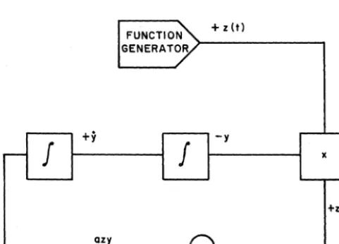
As shown in Figure 1 (a mathematical block dia-gram of the system) the function z (t) must be gen-erated and interjected into the simulation to obtain the solution. There are two possible methods of generating z (t). The first method is to use a diode function generator which approximates the function over a fixed range with straight-line segments. This method is unsatisfactory because of the fixed range restriction-±90° is typical-in addition to the errors introduced by the straight-line approxima-tion of the funcapproxima-tion. It should be noted that special logic circuitry can be programmed in conjunction with the diode function generator to provide a con-tinuous function; however, this only serves to point out the impracticality of this method.
FUNCTION + z (t)
GENERATOR
+y
J
J
-y-
x+zy
azy
[image:2.632.45.286.356.529.2]a
Figure 1. Mathematical Block Diagram
A more accurate and efficient method of generating z (t) is obtained by the solution of a differential equation. The differential equation, which is ob-tained by differentiating equation (6) twice, is
(8)
which has the initial conditions
z (0) == 0 (9)
t It is assumed that the reader ;s familiar with the fundamentals of
analog computation.
2
and
~
==0dt z == 0 (10)
This method is applicable only when the function to be generated is analytic, and a convenient form of its differential equation can be obtained.
The maximum value of z(t) and dz/dt, which was determined while obtaining equation (8), is two. The maximum values of y(t) and dy/dt can be esti-mated by replacing z(t) in equation (7) by its maximum value to obtain a simplified version of Mathieus' equation, namely
o
(11)The solution to this equation-the equation of an oscillator-using the initial conditions defined by equations (2) and (3) is
y(t) == y(o) Cos w t
n (12)
where y (0), the initial value ofy (t), is unity and the frequency of oscillation, W , is
n
w
n 2a
From equation (12) it is obvious that
(13)
(14)
At face value, the maximum value of y (t) is unity; however, since some of the solutions of interest in this study are unstable, y (o)-the estimated maximum value of y (t)-was chosen as five to provide a margin of safety. The maximum value of dy/dt then becomes twenty five, since the maximum value of w is
W
n
n
max
~2a
max~
<
5 (15)and the maximum value of the derivative from equation (14) is y (0) W •
n
TABLE I - MAGNITUDE SCALING SUMMARY
Variable E"timated Scale Computer (Dimensionless) Maximum
(
~~~::r
)
VariableValue (volts)
(Dimensionless) Dim. unit
y 5 2 [2yJ
Y
25 2/5[~
yJ
z 2 5 [5z ]
Z 2 5 [5z ]
The following scaled voltage equationst were ob-tained fo r z and y
d
dt
d
dt
[5z] (16)
= -10 (9) [2y] [5z]
25 10 (17)
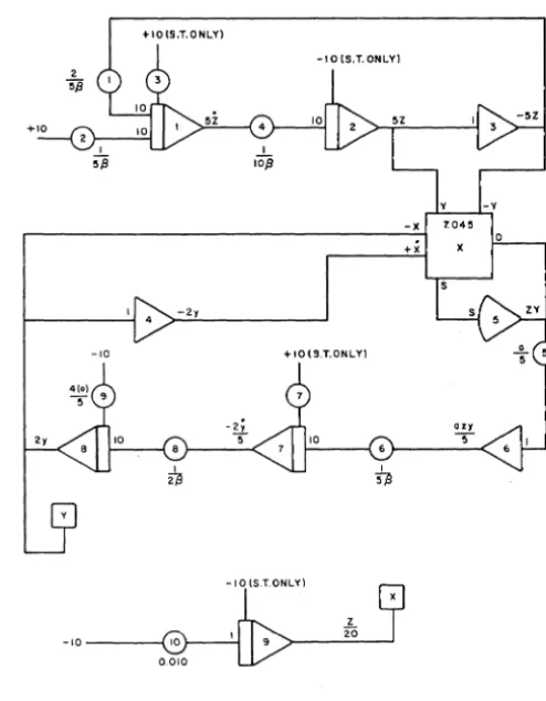
The computer diagram for the simulation is shown in Figure 2 and the potentiometer and amplifier sheets, which include the static check, are shown in Figures 3 and 4. A tabulation of the computing equipment required to perform this simulation is contained in Appendix B.
r-____________________________________ -~x 7.04~
+x
-2,
-10 +IO(9.T.ONLYI
-IO(S.T.ONLY\
-10 - - - {
z 20
Figure 2. Computer Diagram
t [ ] = reference or computer vortage ( ) = potentiometer setting
10, 7, etc. = input gain
3
The time scale factor, {3, was selected as one half so that as much of the solution as possible could be examined in a reasonable length of time (100 seconds). This selection of {3 was governed also by the potentiometer settings which could not exceed one.
PROBLEM Mathieus' Eq.
POT PARAMETER SETTING STATIC CHECK SETTING NOTES POT
NO DESCRIPTION STATIC OUTPUT RUN NO.
CHECK VOLTAGE NUMBER I
2/5~ 0.800
list! 0,400
Constant 0.200
l/lO(j 0.200
a/5 0.500 Parametric Varia.ble
1/56 0.200 (lADO ~
, Constant O. :100
1/213 0,300 1. OUO ~
y(0)/5 o. eoo 0.200 ~
10. Const.'1nt 0.010
Figure 3. TR-10 Potentiometer Assignment Sheet
PROBLEM Mathicus' Eg.
AMP I OUTPUT STAne CHECK
NQ FO VARIABLE CALCl.l..ATEO WEASURED NOTES OUTPUT
I N -5z 4.00' -2.00
, NT 5, 4.00 10.00
, Su, -5' -10.00
4 U, -2y -8.00
,
"G 'Y 8.006 S U ---,----azy -4.00
7 I NT - "5 2. y 8.00 -3.00
•
INT 2y 9.00 8.00 9 INT t/20 0.10 10.00
* 10K Feedback in Check Amplifier
Figure 4. TR-10 Amplifier Assignment Sheet
After exammmg the stability plot of the solution, which is derived in Appendix C and illustrated and tabulated in Appendix B, it was decided that computer runs over the range 0.5:$ a~4.0 in 0.5 increments would produce representative results. In addition, trial and error runs to determine the three transition pOints from stable to unstable solutions in this range must be made.
Results
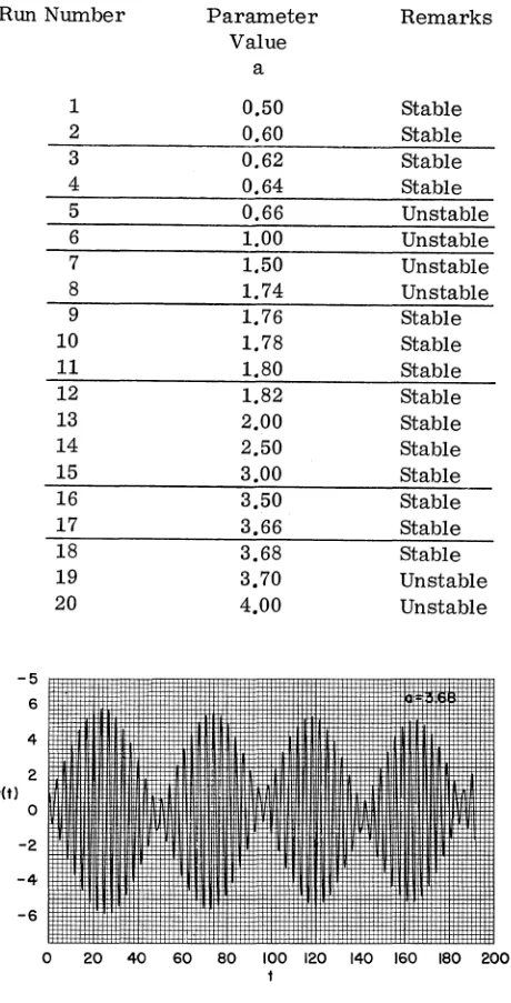
[image:3.621.55.291.49.159.2] [image:3.621.318.557.109.442.2] [image:3.621.49.296.396.713.2]TABLE II. SUMMARY OF COMPUTER RUNS
Run Number
-5 6 4 2 y(t) o -2 -4 -6 1 2 3 4 5 6 7 8 9 10 11 12 13 14 15 16 17 18 19 20 Parameter Value a 0,50 0,60 0,62 0,64 0,66 1.00 1,50 1. 74 1,76 1,78 1.80 1,82 2,00 2,50 3,00 3,50 3,66 3,68 3,70 4,00 Remarks Stable Stable stable Stable Unstable Unstable Unstable Unstable stable stable Stable Stable stable Stable Stable Stable Stable stable Unstable Unstable
o 20 40 60 80 100 120 140 160 180 200
t
Figure 5, y(t) versus t for a=3.68i solution is stable on the verge of being periodic
3 2 o y(t) -I -2
20 40 60 80
Figure 6. y(t) versus t for a=O.50i solution is stable, non-periodic 4 7 6 5 4 3 2 I o
y(t) _I
-2 -3 -4 -5 -6 -7
o 20 40 60 80 100 120 140 160 180 200
Figure 7. y(t) versus t for a=3.70i solution is unstable
8
7
6 STABLE
5
a 4 r--="----_~
3
2
a=2q
.=COMPUTER RESULTS UNSTABLE
O~~~~----~----_L----~----~
o 2
q
Figure 8. Comparison of Theoretical and Computer Results
Conclusions
The objectives of the study have been aChieved. First, the mechanization of Mathieus' equation on the analog computer has been illustrated as well as several noteworthy points regarding function generation, A simple but accurate method of gen-erating an analytic function is from the solution of a differential· equation, which generates the func-tion, This technique presumes that a convenient form of the differential equation can be obtained.
In the case of periodic or sinusoidal functions this is the most practical method of obtaining a con-tinuous function,
Typical solutions, which are cosine elliptic
* ,
of Mathieus' equation are shown in Table I, Runs 1 through 20 (specifically, Figures 5, 6, and 7). [image:4.613.333.561.20.152.2] [image:4.613.69.299.31.483.2] [image:4.613.328.558.208.407.2] [image:4.613.65.297.541.669.2]These non-periodic solutions behave as expected, as "a" increases so does the frequency of the solution, By consulting the literature (5), it was found that the sine elliptic solutions of Mathieus' equation behave in a similar manner, The time required to obtain these results is trivial (less than one hour) when compared to other computa-tional methods,
The percent error of the three computed stability boundary points compared to the literature values(5) is less than 4%, This error is very small when
5
one considers the error usually associated with the parameters used in scientific and engineering studies,
APPENDIX A
TABULATION OF EQUIPMENT
The following major computing components were required to perform this study.
9 Operational Amplifiers
5 Integrator Networks
10 Potentiometers
1 Multiplier
1 X- Y Plotter
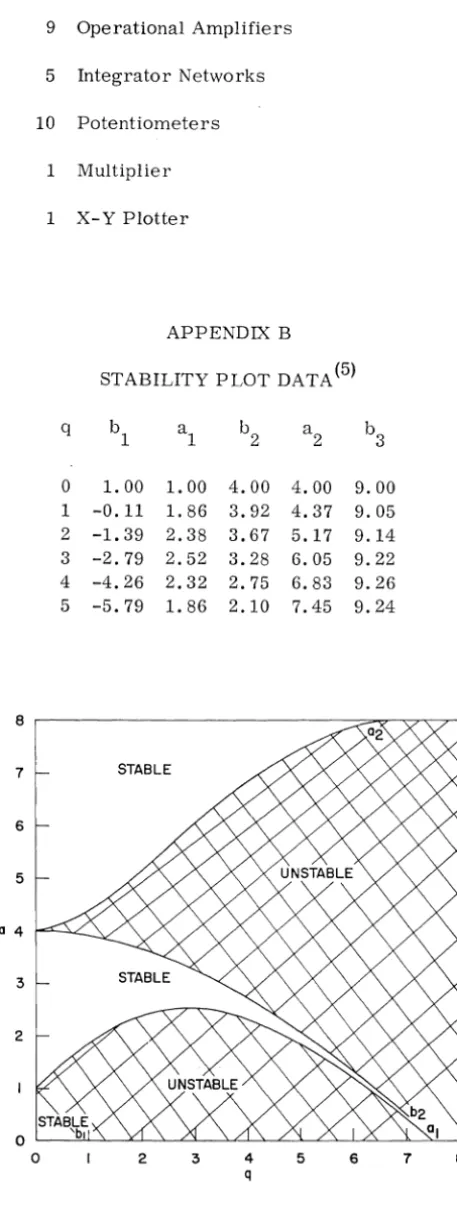
APPENDIX B
STABILITY PLOT DATA (5)
q b 1 a1 b2 a 2 b 3
0 1. 00 1. 00 4.00 4.00 9.00
1 -0.11 1. 86 3.92 4.37 9.05
2 -1. 39 2.38 3.67 5.17 9.14
3 -2.79 2.52 3.28 6.05 9.22
4 -4.26 2.32 2.75 6.83 9.26
5 -5.79 1. 86 2.10 7.45 9.24
8 r---~~~~~
7
6
5
a 4
3
2
2 3 4
q 5
Figure 9. Stability Diagram
6
[image:6.618.189.418.104.709.2]APPENDIX C
ANALYTICAL CONSIDERATIONS OF MATHIE US' EQUATION
One of the more common representations of Mathieus' equation is
2
d y(t) + (a _ 2q Cos 2t) y(t) = 0 2
dt
(1)
where "a" and "q" are constants. The stable
solutions to this equation, which are oscillatory, may be periodic or non-periodic. Fortunately, we need only consider those solutions which are periodic, since the relationships between "a" and "q" on an "a versus q" plot for the periodic so-lutions forms the stability boundaries of the solu-tion(5). The odd and even (sin or cos) solutions to
equation (1) are called Mathieu functions, which
are defined in power series as*
2
cem(t, q) = Cos m t + q c 1 (t) + q c2(t) + ... (2)
and
se (t, q) = Sin m t + q Sl(t) + q2 s (t) + . . . (3)
m 2
where m denotes the order of the function. The "characteristic numbers" of cem and sem are de-noted by am and bm respectively (am and bm are
actually a in equation 1) and are related to "q"
by a power series
2 2 3
am' b m = m + Q 1 q + a 2 q + a 3 q
+...
(4)whose coefficients depend on the order and type of solution.
An "even" solution to equation (1)
y(t) = ce (t, q)
m
is obtained when
y (0) = 1
and
while an "odd" solution
y (t) = se (t,q)
m
* se and ce stand for sine elliptic and cosine el/ipt{c.
(5)
(6)
(7)
(8)
7
is obtained when
y (0) = 0 (9)
and
[dy). _ m
'd
y ) t =0
(10)
A general solution to equation (1) is a linear
com-bination of ce and se
m m
(11)
where A and B are constants of integration.
The coefficients of equation (4) are determined
by substituting either equation (2) or (3) and
equa-tion (4) into equation (1) and solving for the unknown
c or s terms. The a coefficients of equation (4)
are then selected to yield a periodic solution. For example, if m were unity
2
y(t). = Cos t + q c 1 (t) + q c 2(t)
3
+ q c 3(t) +
2 2
d 2y d c 1 2 d c 2
- - = - Cos t + q + q
-dt2 dt2 dt2
2
3 d c3
+ q --2-+
dt
ay(t) Cos t + q[ c 1 (t) + a1 Cos t]+ q [c2 .. 2(t)
(12)
(13)
+ a 1 c1 (t) + a 2 Cos t ] + . " (14)
and
- (2q Cos 2t) = - q (Cos t + Cos 3t)
2
2q c 1 (t) Cos 2 t
-Collecting like powers of q yields
qO Cos t - Cos t = 0
(15)
2
d c1
q --2-+ c (t) - Cos 3t + (a - 1) Cos t = 0 (17)
dt 1 1
and
+ a2 Cos t
=
0 (18)Since the particular in t e g r a I corresponding to
(a1 - 1) Cos t is the non-periodic function 1/2 (1 - (1) t Sin t, 1 is chosen as unity. Therefore,
1
'8
Cos 3 t (19)satisfies equation (17). This method may now be repeated to determine as many terms of the series as desired. The results of the example are
1 1 2
ce1 (t, q) := Cos t -
'8
q Cos 3 t + 64 q (- Cos 3t1
+
'3
Cos 5t) + . . . (20)and
1 2 1 3 1 4
a1 := 1 + q -
'8
q - 64 q - 1536 q +. (21)If the above procedure is repeated for several integral values of "m" a stability plot, which is shown in Figure 9, can be obtained. The data for this plot is tabulated in Appendix B. Only the first quadrant of the stability plot is considered in this study. However, it should be noted that the second quadrant is a minor image of the first quadrant.
LIST OF SYMBOLS
a Parameter Dimensionless
a Characteristic number of ce Dimensionless
m m
b Characteristic number of se Dimensionless
m m
m Order of Mathieu function Dimensionless
q Parameter Dimensionless
y Dependent variable Dimensionless
z Frequency variable Dimensionless
A Constant of integration Dimensionless
B Constant of integration Dimensionless
{3 Time scale factor Seconds
Dimensionless Unit
ce Mathieu function (cosine elllptic) Dimensionless
m
se Mathieu function (sine elliptic) Dimensionless m
REFERENCES
1. Bell, H., Jr.; The Solution of Mathieu's Equa-tion by an Analog Computer; M.S. Thesis; University of Wisconsin, 1951.
2. Den Hartog, J.p.; Mechanical Vibrations; 4th Ed. McGraw-Hill Book Co., Inc.; New York, N.Y.; 1956.
3. Gray, H.J., Merwin, R., and Brainerd, J.G.; Solutions of the Mathieu Equation; AlEE Trans-actions; Vol. 67; 1948.
4. Margenau, H. and Murphy, G.M.; Mathematics of Physics and Chemistry; D. Van Nostrand Co., Inc.; New York, N.Y.; 1956.
5. McLachlan, N.W.; Theory and Application of Mathieu Functions; Oxford University Press; London; 1947.
6. Minorsky, N.; Non-Linear Vibrations; Edwards Brothers, Inc.; Ann Arbor, Michigan; 1947.
7. Stoker, J.J.; Nonlinear Vibrations; Interscience Publishers, Inc.; New York, N.Y.; 1954.
8. Whittaker, E. T. and Watson, G.N.; Modern Analysis; Cambridge University Press; New York, N,Y,; 1927,
EAI
4DELECTRONIC ASSOCIATES, INC. Long Branch, New Jersey