https://doi.org/10.5194/hess-21-5043-2017 © Author(s) 2017. This work is distributed under the Creative Commons Attribution 3.0 License.
Identifying, characterizing and predicting spatial patterns of
lacustrine groundwater discharge
Christina Tecklenburg and Theresa Blume
Helmholtz Centre Potsdam, GFZ German Research Centre for Geosciences, Department of Hydrology, Potsdam, Germany Correspondence to:Theresa Blume ([email protected])
Received: 29 November 2016 – Discussion started: 13 December 2016 Revised: 28 July 2017 – Accepted: 31 July 2017 – Published: 6 October 2017
Abstract.Lacustrine groundwater discharge (LGD) can sig-nificantly affect lake water balances and lake water quality. However, quantifying LGD and its spatial patterns is chal-lenging because of the large spatial extent of the aquifer– lake interface and pronounced spatial variability. This is the first experimental study to specifically study these larger-scale patterns with sufficient spatial resolution to system-atically investigate how landscape and local characteristics affect the spatial variability in LGD. We measured vertical temperature profiles around a 0.49 km2 lake in northeast-ern Germany with a needle thermistor, which has the ad-vantage of allowing for rapid (manual) measurements and thus, when used in a survey, high spatial coverage and res-olution. Groundwater inflow rates were then estimated us-ing the heat transport equation. These near-shore temper-ature profiles were complemented with sediment tempera-ture measurements with a fibre-optic cable along six tran-sects from shoreline to shoreline and radon measurements of lake water samples to qualitatively identify LGD patterns in the offshore part of the lake. As the hydrogeology of the catchment is sufficiently homogeneous (sandy sediments of a glacial outwash plain; no bedrock control) to avoid patterns being dominated by geological discontinuities, we were able to test the common assumptions that spatial patterns of LGD are mainly controlled by sediment characteristics and the groundwater flow field. We also tested the assumption that topographic gradients can be used as a proxy for gradients of the groundwater flow field. Thanks to the extensive data set, these tests could be carried out in a nested design, consider-ing both small- and large-scale variability in LGD. We found that LGD was concentrated in the near-shore area, but along-shore variability was high, with specific regions of higher rates and higher spatial variability. Median inflow rates were
44 L m−2d−1with maximum rates in certain locations going
up to 169 L m−2d−1. Offshore LGD was negligible except for two local hotspots on steep steps in the lake bed topogra-phy. Large-scale groundwater inflow patterns were correlated with topography and the groundwater flow field, whereas small-scale patterns correlated with grain size distributions of the lake sediment. These findings confirm results and as-sumptions of theoretical and modelling studies more system-atically than was previously possible with coarser sampling designs. However, we also found that a significant fraction of the variance in LGD could not be explained by these controls alone and that additional processes need to be considered. While regression models using these controls as explanatory variables had limited power to predict LGD rates, the results nevertheless encourage the use of topographic indices and sediment heterogeneity as an aid for targeted campaigns in future studies of groundwater discharge to lakes.
1 Introduction
1.1 Spatial patterns of lacustrine groundwater discharge and their potential controls
In an isotropic homogenous aquifer, the exchange between groundwater and lake is expected to follow a distinct pat-tern along a 2-D transect: as sloping groundwater water tables meet the flat surface of the lake, groundwater in-flow is strongest in close proximity to the shoreline and de-creases exponentially with distance to the shore (McBride and Pfannkuch, 1975). However, isotropic and homogenous conditions rarely exist and spatial distribution of ground-water inflow differs strongly from lake to lake (Rosenberry et al., 2015). Experimental studies highlighted a large variety of observed exchange patterns including decreasing seepage with distance from the shoreline (McBride and Pfannkuch, 1975; Brock et al., 1982; Cherkauer and Nader, 1989; Kishel and Gerla, 2002), increasing seepage with distance from the shoreline (Cherkauer and Nader, 1989; Schneider et al., 2005; Vainu et al., 2015), local hotspots of offshore seepage (Fleckenstein et al., 2009; Ono et al., 2012) and a high small-scale variability in near-shore zones (Kishel and Gerla, 2002; Blume et al., 2013; Neumann et al., 2013; Sebok et al., 2013). Most often, complex hydrogeological settings are the reason for deviations from the theoretical pattern of LGD (Rosen-berry et al., 2015). For example, it was found that offshore LGD was caused by local connections with a deeper aquifer (Fleckenstein et al., 2009; Ono et al., 2012) or resulted from local thinning of low permeable lake sediment (Cherkauer and Nader, 1989).
In general, the position of a lake in its regional ground-water flow system determines if a lake receives groundwa-ter, loses water towards the groundwater or both (Born et al., 1979). As the groundwater flow field is often not well known, landscape topography can help to determine the groundwa-ter flow field in humid regions and homogenous aquifers, where groundwater tables are assumed to follow the topog-raphy (Toth, 1963). However, Haitjema and Mitchell-Bruker (2005) found that the groundwater table is only topograph-ically controlled if the ratio of groundwater recharge over hydraulic conductivity is sufficiently large and that often groundwater tables are indeed not topography, but recharge controlled (for a US-wide classification of these groundwater table controls, see also Gleeson et al., 2011).
Little is known about controls of small-scale variability of LGD. LGD is driven by the hydraulic gradients between lake and aquifer and controlled by the hydraulic conduc-tivity. So far, there is no clear picture about the role of lake sediment characteristics in controlling LGD patterns and observations seem to be very site specific. For example, Kidmose et al. (2013) found that low permeable lacustrine sediments can completely prevent groundwater upwelling, whereas Vainu et al. (2015) observed LGD through low per-meable lacustrine sediments. Kishel and Gerla (2002) asso-ciated small-scale variabilities in LGD with small-scale het-erogeneities in hydraulic conductivities (Kishel and Gerla,
2002); Schneider et al. (2005) found no correlation between seepage rates and sediment characteristics.
Methods used in these studies include seepage meters (e.g. Kidmose et al., 2013; Kishel and Gerla, 2002; Schneider et al., 2005; Vainu et al., 2015) and piezometers (Kishel and Gerla, 2002). Two other methods have also been used successfully to investigate exchange patterns between lakes and groundwater: fibre-optic distributed temperature sens-ing (FO-DTS) (Blume et al., 2013; Sebok et al., 2013) and vertical temperature profiles (VTPs) (Blume et al., 2013; Meinikmann et al., 2013; Neumann et al., 2013; Sebok et al., 2013). Both methods use heat as a tracer. The measurement of radon activities can also help to identify groundwater in-flows (Kluge et al., 2012; Ono et al., 2012; Shaw et al., 2013). Existing lake studies have investigated LGD patterns with either a high spatial resolution (1–2 m2) but a local focus (10 m×17 m–25 m×6 m) (Kishel and Gerla, 2002; Blume et al.; 2013; Sebok et al., 2013) or focused on the entire lake but used a relatively low spatial resolution (measurements along the shoreline every 200–3000 m) (Schneider et al., 2005; Meinikmann et al., 2013; Shaw et al., 2013). However, the experimental effort required rarely allows their extension to cover the lateral, alongshore dimension in sufficient extent and detail to identify the spatial variability and patterns of LGD along the shoreline.
1.2 Objectives
Identifying the processes and structures controlling LGD pat-terns is the key to predicting them reliably (Grimm, 2005). The aim of this study is the characterization of inflow pat-terns as well as the identification of their controls. The abil-ity to identify patterns and their controls strongly depends on the spatial resolution and the extent of the applied experi-mental methods. By taking measurements with a high spatial resolution over large parts of the lake, we are closing the ob-servational gap between high-resolution “plot”-scale studies (focusing on a small shoreline segment) and low-resolution larger-scale studies (see Sect. 1.2) and opening the possibil-ity to truly investigate not only shore–lake transects or plots but alongshore spatial variability and patterns of LGD.
The study design aimed at answering the following re-search questions:
– How does LGD vary in space and time?
– What are the relative roles of sediment permeability, lo-cal topography and regional groundwater discharge for spatial patterns of LGD?
– Can we use LGD patterns to test if groundwater tables are topography controlled?
in the last decades at this lake as well as at others in the re-gion are currently under investigation. This lake system has the additional advantage that the upper unconfined aquifer in which the lake rests can be considered largely homogeneous and isotropic (sandy sediments of a glacial outwash plain; no bedrock control). Therefore, LGD patterns are unlikely to be dominated by geological discontinuities, and we were able to test the common assumptions that spatial patterns of LGD are controlled by sediment characteristics and topography as a proxy for gradients of the groundwater flow field.
To identify LGD patterns, we measured VTPs in the near-shore area and used FO-DTS measurements and radon sam-pling in the offshore area. VTPs were used to quantify LGD rates, whereas FO-DTS measurements and radon sampling were used as qualitative tracers to detect the presence or ab-sence of offshore LGD.
2 Methods 2.1 Study site
Lake Hinnensee is located in northeast Germany in the Müritz National Park (53◦19030.600N, 13◦11016.200E) and is one of the focus areas of the TERENO observatory north-east Germany. The landscape of the Müritz National Park was shaped by the last glaciation and is dominated by lakes. Lake Hinnensee was formed as a glacio-fluvial tunnel val-ley and is located within the outwash plain. Bore logs of the 16 observation wells installed around the lake show largely homogeneous sandy sediments. The terminal moraine is sit-uated north of the lake (Fig. 1). Lake Hinnensee has a mean depth of 7 m with a maximum depth of 14 m and is connected to a lake called Großer Fürstenseer See in the south. The two lakes together cover an area of 2.68 km2; the size of Lake Hinnensee is 0.49 km2. The lake system has no surface water inflow or outflow, apart from a two minor ditches connected with the Großer Fürstenseer See that only become active at very high lake level. Since 2011, when the first LGD mea-surements were conducted at Lake Hinnensee, the ditches were only active for a period of 4 months (maximum ob-served inflow: 0.0083 m3s−1, 22 February 2012; maximum observed outflow: 0.0030 m3s−1, 11 May 2012). The con-nection to Großer Fürstenseer See is not assumed to influ-ence LGD patterns of Lake Hinnensee, as the general flow direction of the groundwater flow field runs from north to south, with water leaving the lake system at the southern end of Großer Fürstenseer See. The relief of the lake catchment is hilly in the north, with steep slopes down to the lake and more gentle slopes and lower elevations towards the south (Fig. 1). Elevations range between 63 and 115 m a.s.l. The lake is surrounded by forest. The mean annual precipitation is 610 mm and the mean annual temperature is 8.1◦C (1901– 2005 Neustrelitz, DWD – German Weather Service).
2.2 Estimating lacustrine groundwater discharge We applied three different methods to determine LGD pat-terns: VTPs in the near-shore region, and FO-DTS and radon in the offshore area. The VTPs allowed us to determine LGD rates by using the analytical solution of the heat transport equation, while the other methods were only used as indica-tors for the presence and absence of LGD. As the main body of the study focuses on the temperature-based methods, the radon methodology and results are described in Appendix A. 2.2.1 Near-shore LGD derived from vertical
temperature profiles (VTPs)
VTPs were used to estimate the spatial variability of LGD rates along the shoreline. Profiles were measured 50 cm away from the shoreline every 10 m along 2.39 km of the shore-line. The data set covers 62 % of the total shoreline (Fig. 1). The VTPs were measured during five field campaigns in Au-gust 2011, June and July 2012, and January and July 2013 (Table 1, Fig. 1). In July 2013, sediment temperatures were additionally measured in 150 cm distance from the shoreline in order to analyse the trend of LGD with increasing dis-tance to the shore. Measurements in August 2011 and Jan-uary 2013 were conducted only on a 350 m long subsection of the shoreline in the northeast of the lake in order to analyse the temporal stability of the observed patterns (Fig. 1).
One VTP consisted of six temperature measurements: one at the sediment–water interface and five in the saturated sediment at 5, 10, 20, 30, and 40 cm depths. Temperatures were measured with a high-precision digital thermometer (Greisinger GMH 3750) and a corresponding Pt100 thermis-tor with an accuracy of±0.03◦C. The needle had a length of 45 cm and a diameter of 3 mm.
LGD was calculated from the measured VTP using the analytical solution of the 1-D heat flow equation from Bre-dehoeft and Papaopulos (1965). Assuming a vertical water flux along the temperature profile and steady-state tempera-tures at the sediment–water interface, sediment temperature at a specific depth is calculated as follows:
Tmod(z)= exp
qz·pfcf·z kfs −1
exp
qz·pfcf·L kfs −1
·(TL−T0)+T0, (1)
where qz is the vertical water flux (m s−1) (positive for groundwater gaining),pfcf is the volumetric heat capacity
of the fluid (J m−3K−1), z is the depth below the upper
boundary (m),kfsis the thermal conductivity of the sediment
(J s−1m−1K−1),L is the extent of the exchange zone and the depth of the lower boundary (m), andTLis the
temper-ature of the lower andT0 of the upper boundary (◦C). The
values ofpfcfof water andkfsof lake sediment were taken
from Stonestrom and Constantz (2003).pfcfof water was set
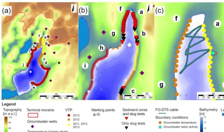
Figure 1.Study site and experimental infrastructure.(a)Overview of the study site with VTP measurement and locations of groundwater wells and temperature logger chains,(b)slug test and sediment core sampling locations and(c)FO-DTS cable installation in the northern part of the lake.
Table 1.Dates, boundary conditions and use of vertical temperature profile surveys.
Date Groundwater Lake water Data analysis temperature (◦C) temperature (◦C)
24–25 Aug 2011 10.7 22.7 Temporal stability of LGD patterns 12–14 Jun 2012 8.9 18.2 Spatial patterns of LGD along the shoreline 16–17 Jul 2012 10.1 20.1 Spatial patterns of LGD along the shoreline 21–23 Jan 2013 7.0 0.0 Spatial patterns of LGD along the shoreline
17–25 Jul 2013 10.1–10.3 23.2 Spatial patterns of LGD along the shoreline and LGD patterns with increasing distance from the shore
value for sandy sediment, which was the dominant grain size in the upper metre of lake sediment.
Usually, the upper boundary is the sediment–water inter-face (Schmidt et al., 2006; Blume et al., 2013; Meinikmann et al., 2013). However, at locations with shallow water depths in lakes, temperatures in the near-surface sediments can be strongly affected by daily temperature variations and thus vi-olate the upper boundary condition of the steady-state model. To avoid unreliable LGD calculations due to biased temper-atures at the upper boundary, we instead used the tempera-tures measured at 10 cm sediment depth. A shift of the up-per boundary from the sediment–water interface to a depth of 10 cm had a negligible effect on the estimation of the LGD rate assuming steady-state conditions. This was val-idated with theoretical temperature profiles. A shift of the boundary condition to a depth of 10 cm caused a maximal deviation in the estimation of exchange rates of 1 L m−2d−1 and the error decreased with increasing flow rates.
For the lower boundary, we used the shallow ground-water temperature measured in close proximity to the lake (Fig. 1c). For the length of the exchange zone, we tested dif-ferent values. The quality of LGD estimation increased with increasingLbut was insensitive for values larger than 3 m. Thus,Lwas set to 3 m.
The exchange rate was optimized by minimizing the root mean square error (RMSE) between measured and calculated sediment temperatures, as described in Schmidt et al. (2006):
RMSE=
r
1 n
X
Tmeas(z)−Tmod(z)
2
. (2)
[image:4.612.86.507.363.463.2]Estimated LGD values were analysed for their lateral spa-tial variability using VTPs measured at a distance of 50 cm from the shoreline, for their trend with increasing distance from the shore using VTPs measured at 50 and 150 cm dis-tances from the shore and for their temporal stability using VTPs measured in the different years (Table 1).
Spatial variability and correlation of LGD along different distances along the shoreline were analysed using autocor-relation plots and autocorautocor-relation values (|ρ|) as described in Caruso et al. (2016). High autocorrelation indicates that LGDs along a given stretch of the shoreline are correlated (i.e. if LGD is high in a certain location, it is also likely to be high at 10 m distance), whereas|ρ|<0.2 indicates that LGDs are uncorrelated and strong spatial variability exists.
In order to analyse the temporal stability of spatial pat-terns, we used the differences between the LGD rates mea-sured at different points in time and calculated the correlation between the VTP surveys using Spearman’s rank correlation coefficient (ρ). Correlations were regarded as significant for pvalues smaller than 0.05.
To test if single sediment temperature measurements in-stead of profiles could be used as a quickly measurable qual-itative indication for LGD spatial patterns, we determined the correlations between sediment temperatures at all individual depths with LGD rates determined from the full profiles. 2.2.2 Lake sediment temperature anomalies as
indicators for offshore LGD based on fibre-optic distributed temperature sensing (FO-DTS) To identify offshore groundwater inflow patterns, we mea-sured sediment surface temperatures with a 500 m long FO-DTS cable installed permanently along six transects through the northern part of the lake (Fig. 1c). Two divers ensured good contact of the cable to the lake sediment and also tracked the location of the cable with a differential GPS sys-tem (Topcon GR-3) installed on a buoy.
The technology of the FO-DTS is based on the detection of the Raman scattering of a laser pulse through the opti-cal fibre (Ukil et al., 2012). For our measurements, we used a Sensornet Halo device with a sampling resolution of 2 m and a measurement precision of 0.05◦C.
We carried out two measurement campaigns: in February and in August 2014 (Table 2). In February, the DTS mea-surements were taken between 18:49 and 19:17 CEST with a temporal resolution of 2 min. We used a single-ended set-up with a double-ended mode (four channels, two in each direction) and two calibration baths: a warm bath (25.5◦C) at one end and a cold bath (0◦C) at the other end.
In the second campaign, from 27 to 28 August 2014, mea-surements extended over 24 h, from 18:43 on the 27th un-til 18:45 CEST the next day with a temporal resolution of 2 min. The setup was the same as in February, but addition-ally both cable ends were run through the cold bath (warm bath: 20.9◦C; cold bath: 0.1◦C).
The trend and offset in the DTS temperature data were corrected using external temperature loggers in the cali-bration baths (February: Greisinger GMH 3750, accuracy:
±0.03◦C; August: HOBO TidbiT v2 water temperature data logger, accuracy:±0.21◦C).
All four channels showed the same pattern with only small differences in absolute temperature values, and further anal-yses were based on one of the four traces. Sediment temper-atures in August were strongly affected by solar radiation. Analysis of 24 h amplitude or daily minimum temperature did not provide useful information of groundwater inflow patterns as the impact of solar radiation was too strong and spatially variable. Sebok et al. (2013) recommended using nighttime data to avoid the uncertainties caused by solar ra-diation. However, at night, shallow near-shore water cooled down and it was not easy to distinguish if temperature shifts resulted from groundwater inflow or from a decrease of water temperature due to decreasing air temperature. We thus chose a time window in which the temperatures at the near-shore shallow region and in the deeper region of the lake were very similar and groundwater inflow induced temperature shifts were easy to identify. This time window was from 18:43 to 19:11 CEST on 27 August.
Temperature depth profiles of the lake were available with 1 m spatial resolution (HOBO Water Temperature Pro v2 data logger, accuracy: ±0.21◦C). In winter, we had only one profile in the central part of the lake, but in August a second profile further north was available (Fig. 1a and b). The groundwater temperature was measured in a piezome-ter (OTT Orpheus Mini, accuracy: ±0.5◦C) close to the lake (Fig. 1c) and air temperature data were available from a weather station 1.5 km away, and in August an additional air temperature data logger (of the same type as used for the water profiles) was installed directly at the lake.
2.3 Identifying controls of LGD patterns
In order to identify the controls of the observed LGD pat-terns, we characterized both the near- and far-field condi-tions and correlated these characteristics with LGD rates us-ing Spearman’s rank correlation coefficient. At the local scale (near-field conditions) this includes sediment characteristics, while at the larger scale (far-field conditions) we considered topographic indices and the groundwater flow field as the most likely controls.
2.3.1 Sediment heterogeneity as a small-scale control on LGD patterns
Hydraulic conductivity from slug tests
At 37 VTP positions (Fig. 1b), slug tests were performed to estimate hydraulic conductivity (ksat) of the near-surface
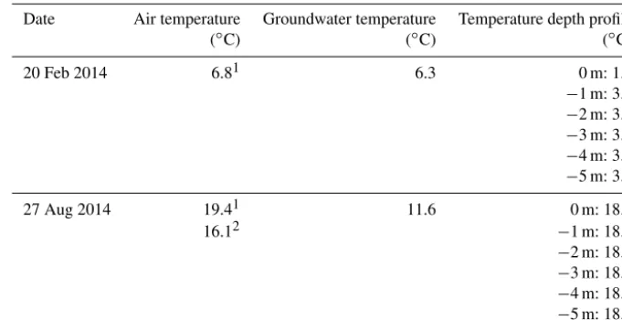
Table 2.Groundwater temperatures and lake water temperature depth profiles measured during FO-DTS campaigns.
Date Air temperature Groundwater temperature Temperature depth profile
(◦C) (◦C) (◦C)
20 Feb 2014 6.81 6.3 0 m: 1.8
−1 m: 3.4
−2 m: 3.4
−3 m: 3.4
−4 m: 3.4
−5 m: 3.4
27 Aug 2014 19.41 11.6 0 m: 18.9
16.12 −1 m: 18.7
−2 m: 18.7
−3 m: 18.5
−4 m: 18.4
−5 m: 18.4
1Measured at the nearby weather station.2Measured close to the lake.
end of the piezometer had a length of 10 cm and consisted of 4 mm diameter perforations in the PVC tube wrapped with fine mesh. The midpoint of the screen was 50 cm below the sediment surface. To minimize interference with the temper-ature profile measurements, the piezometers were installed at 50 cm distance. For the rising-head tests, water was quickly removed out of the piezometer using a peristaltic pump. Re-covery of the water table was measured with automatic pres-sure logger (HOBO 13 ft freshwater level data logger, ac-curacy:±0.3 cm) with a temporal resolution of 1 s. Recov-ery data were then analysed using the approach of Hvorslev (1951):
ksat= π r2 T0c
, (3)
whereris the radius of the piezometer,T0the time needed to
recover 37 % of initial water level andca shape factor. The shape factor depends on the ratio of screen length and radius. The piezometer had a screen length radius ratio of 5.5, and thus we used a shape factor introduced by Chapuis (1989), valid for wells with ratio smaller than 8:
c=4π r
r
L 2r +
1
4, (4)
whereLis the length of the screen.
Grain size distributions from sediment cores
Sediment cores were taken from 30 selected slug test po-sitions (Fig. 1b). Sediment cores were taken with a trans-parent tube with an inner diameter of 32 mm. The length of cores varied between 42 and 145 cm, with the major-ity of core lengths between 80 and 128 cm. Each core was split into samples according to the visible sediment layers. The samples were oven-dried at a temperature of 105◦C
and sieved with a vibratory sieve shaker (Retsch AS 200). The sieving setup included the following mesh sizes: 0.063, 0.125, 0.2, 0.3, 0.5, 0.63, 2, 5 and 10 mm. Grain sizes smaller than 0.063 mm were classified as silt, grain sizes larger than 0.063 mm but smaller than 0.2 mm as fine sand, larger than 0.2 mm but smaller than 0.63 mm as medium sand, larger than 0.63 mm but smaller than 2 mm as coarse sand and larger than 2 mm as gravel.
For the correlation analyses between sediment character-istics and LGD, we used only samples taken from the upper 100 cm of the lake sediment. The mean of each grain size fraction was calculated for each sampling location from all single samples of the upper 100 cm in which the core was split. In addition to the correlation analyses, simple and mul-tiple linear regression models were calculated between LGD and each grain size fraction. For the calculation of the mul-tiple linear regression models, correlations between explana-tory variables were checked before and variables were re-garded to be independent from each other ifρ was below 0.7. Models were regarded as significant ifpvalues were be-low 0.05. The goodness of fit of the models was estimated with the coefficient of determination (R2).
2.3.2 Topographic indices as controls on large-scale LGD patterns
split into 46 subsections of 100 m length with an overlap of 50 m. As upslope areas can only be determined for points, not for lines, we calculated upslope areas every metre along the shoreline and aggregated them to one upslope area for each subsection. The upslope areas were determined using the multiple flow direction approach. To investigate the topo-graphical zone of influence (zi), four different extents of the upslope areas were considered at 25, 50, 100 and 200 m dis-tances from the shoreline. These zones of influence will be called zi25 m, zi50 m, zi100 mand zi200 min the following. The
indices’ slope and elevation were averaged over each upslope area (arithmetic mean). The percentage of area with low to-pographic gradient was here defined as the percentage of the upslope area not to be higher than 50 cm above lake level in direct vicinity of the lake shore. This threshold was chosen as this was the area flooded at maximum lake levels known within the last 25 years. Indices were correlated with median LGD rates for the 100 m long subsections derived from VTPs using Spearman’s rank correlation coefficient. Each subsec-tion included 10 VTP measurement locasubsec-tions. Furthermore, simple and multiple linear regression models were calculated between LGDs and topographic indices derived for zi25 m
and zi50 m, as in these zones correlation between LGD and
far-field conditions was strongest. Correlations between ex-planatory variables were checked and regarded as indepen-dent from each other ifρwas below 0.7. Predictors were re-garded as significant ifpvalues were below 0.05. The good-ness of fit of the models was estimated based on the coeffi-cient of determination (R2).
2.3.3 Groundwater flow field as control on large-scale LGD patterns
The groundwater flow field was the second far-field vari-able assumed to affect the LGD patterns. The groundwater flow field is generally assumed to be largely controlled by topography. We used two approaches to test this assump-tion: the water table ratio (Haitjema and Mitchell-Bruker, 2005) and a comparative analysis of flow fields determined based on measured groundwater levels alone (ordinary krig-ing) or including topographic effects (regression krigkrig-ing). The simple dimensionless water table ratio (WTR) is equal to (RL2)/(mkH d), withRas the annual recharge rate (m d−1), L as the mean distance between surface waters (m),m=8 or 16 (–) for either 1-D or radial flow, k as the average hydraulic conductivity (m d−1), H as the average aquifer thickness (m) andd as the maximum terrain rise (m) (Hait-jema and Mitchell-Bruker, 2005; Gleeson et al., 2011) al-lows a first test of the potential influence of topography on the groundwater flow field, with WTR greater than 1 indicat-ing topography-controlled water tables and WTR less than 1 indicating recharge-controlled water tables. The average hy-draulic conductivities were determined from 92 undisturbed cores taken during observation well installation and were measured in the lab using a permeameter.
In order to derive the groundwater flow field, measured groundwater heads from 16 observation wells located around Lake Hinnensee (Fig. 1a) were spatially interpolated. A to-tal of 12 of the 16 bore wells were drilled in 2012, 3 were drilled in 2014 and 1 existed already before installation of the TERENO monitoring network. Groundwater levels were measured every 7–9 weeks since 2012 using an electric con-tact meter (SEBA Hydrometrie, electric concon-tact meter type KLL, accuracy:±1 cm). To determine the groundwater flow field, we used groundwater levels measured in 2014, when all wells were completed. In 2014, groundwater levels were gen-erally lower than during the VTP measurement campaigns (2011–2013), but the spatial patterns of groundwater heads of the 12 wells already installed in 2012 remained stable. Groundwater levels from March 2014 had the smallest dif-ferences (mean difference 5.55 cm) to available groundwater data around the time of the VTP measurement campaigns and were thus chosen to derive the groundwater flow field. For the interpolation of the groundwater measurements, we used both ordinary kriging and regression kriging. In regression kriging, a linear regression between an external variable and the depending variable is included. This allowed us to incor-porate the potential effect of topography on the groundwater flow field. In order to minimize the effect of small-scale het-erogeneities in the topography, the DEM was smoothed by reducing the resolution from 1 to 10 m and rescaling to a res-olution of 1 m to maintain a consistent resres-olution of the re-sults. The groundwater gradients were then calculated from the interpolated groundwater surface.
To analyse the correlation of the groundwater flow field with the LGD patterns, we averaged groundwater gradients in each of the subcatchments for each zone of influence (arithmetic mean) and correlated these with the median LGD rates of the subsections using Spearman’s rank correlation coefficient as described in Sect. 2.3.2. In addition to the cor-relation analyses, simple linear regression models were cal-culated between LGD and groundwater gradients. Further-more, groundwater gradients were also included in multiple linear regression models with topographic indices.
All analyses were carried out in the statistic software R (R Development Core Team, 2011). For the geographi-cal analyses, we used the geographigeographi-cal information system SAGA GIS and the package “rsaga” (Brenning, 2008).
3 Results
3.1 Estimating lacustrine groundwater discharge 3.1.1 Near-shore LGD derived from vertical
temperature profiles
with increasing distance from the shore and (c) the tempo-ral stability of LGD patterns. These 520 profiles thus include repeated measurements in time as well as measurements at two distances to the shore. At the western lake section, 150 to 290 m from the northern tip, VTP measurements could only be taken every 20 m instead of every 10 m as the lake shore could either not be accessed or the sediment was unsuitable for measuring due to a thick layer of muddy organic mate-rial. However, as lake sediments in this lake section were quite homogeneous, we assume that despite the wider spac-ing we still captured the spatial variability of LGD. The same reasons also precluded measurements at 11 other locations around the lake. These other 11 locations were irregularly distributed so that gaps were small and we do not expect a strong influence of these gaps on overall spatial patterns. A total of 22 profiles (4 %) were excluded from the analy-ses as no satisfying fit to the heat transport equation could be achieved. The quality of all remaining LGD estimations was satisfactory (median(RMSE)=0.06◦C;n=498).
Spatial patterns along the shoreline
LGD rates determined from VTPs every 10 m along 2.39 km of the shoreline (216 locations) ranged from
−12 L m−2d−1(losses) to 169 L m−2d−1(gains) with a me-dian of 44 L m−2d−1 and an interquartile range (IQR) of 26 L m−2d−1. Occurrence of very strong LGD rates of more than 94 L m−2d−1 (positive outliers of LGD distribution) was limited to the northernmost 140 m on both the western and eastern shores of the lake (between “a” and “b” and “f” and “g” in Fig. 2b and c) and to one single spot at the western shore 470 m to the south (“i” in Figs. 1 and 2c). The north-ernmost 140 m on both the western and eastern shores (be-tween “a” and “b” and “f” and “g” in Figs. 1 and 2b, c) are in the following called “the northern part” and the adjacent region in the south (between “b” and “e” and “g” and “j” in Figs. 1 and 2b) will be called “the southern part”. Neg-ative rates were only observed at the eastern shore between 480 and 530 m from the northern tip (“c” in Figs. 1 and 2b, c). In the northern part of the lake, LGD was stronger and spatially more variable (median of 74 L m−2d−1) than in the southern part (median of 41 L m−2d−1) (Figs. 2 and 3). In the northern part, LGD was statistically uncorrelated for all lag distances, while in the southern part it was autocorrelated up to a lag distance of 50 m with|ρ| ranging between 0.62 and 0.23 (Fig. 3). Autocorrelation in the southern part was stronger on the eastern than on the western shore.
Spatial patterns perpendicular to the shoreline
Between 660 and 1520 m along the eastern shore and 300 and 830 m south of the northern tip along the western shore, VTPs were measured at 50 and 150 cm distance from the shoreline to analyse the trend of LGD with increasing dis-tance from the shore.
In more than two-thirds of all cases (71 %), LGD measured at 150 cm from the shoreline was lower than the rate mea-sured at 50 cm distance (Fig. 2). The reduction of LGD rate was on average 20 % (median). However, in 29 % of all cases, LGD increased with distance to the shore (Fig. 2) with an av-erage increase of 15 % (median). The patterns of LGD along the shoreline measured 50 and 150 cm apart from the shore were very similar (ρ=0.81(pvalue<2×10⁻¹⁶); Fig. 2). Temporal stability of spatial patterns
The annual repetitions of LGD rates measured at 43 VTP positions (Fig. 1) highlight that the observed LGD pat-terns were correlated between the individual measurement campaigns (Fig. 4). The correlation coefficient was 0.71 (pvalue=5×10⁻⁶) between summer 2011 and 2012 (n=
34), 0.82 (pvalue=10−3) between 2012 and summer 2013 (n=13), 0.70 (pvalue<4×10⁻⁶) between 2012 and win-ter 2013 (n=34), and 0.66 (pvalue<3×10⁻⁵) between 2011 and winter 2013 (n=33). The differences between LGD rates measured in different years were lowest compar-ing rates from summer 2011 and summer 2012 (median of
−6 L m−2d−1) and strongest comparing rates from summer 2011 and winter 2013 (median of 27 L m−2d−1).
Single sediment temperature measurements as a qualitative indicator for LGD spatial patterns
Sediment temperatures from the top of the sediment down to a depth of 10 cm were not well correlated with LGD rates, but strong correlations were found between LGD rates and sediment temperatures measured 20 cm below the surface and deeper (correlation coefficients range between 0.46 and 0.96). While the correlation is generally high, the slope of the regression line varies in time (Fig. 5).
3.1.2 Lake sediment temperature anomalies as indicators for LGD based on fibre-optic distributed temperature sensing (FO-DTS) We measured lake sediment temperature with a FO-DTS ca-ble installed in six transects through the northern part of the lake (Fig. 1c) during two measurement campaigns (20 Febru-ary and 27 August 2014) to identify offshore groundwater in-flow. The complementary results of the radon measurement campaigns are described in Appendix A.
Figure 2.LGD estimated from VTPs measured at 50 and 150 cm distance from the shoreline: LGD distribution from VTPs in the northern and southern parts measured at a distance of 50 cm(a), LGD along the eastern shore(b)and LGD along the western shore(c). Locations where fits of the heat transport equation were poor (RMSE>0.4) are indicted with squares.
Figure 3.Correlation between neighbouring LGD measurement locations (distance 10 m) in the northern part(a)and southern part(b); autocorrelogram for the LGD series of the northern and southern parts of the lake(c).
temperatures and temperature depth profiles of the lake mea-sured during the DTS measurements are presented in Table 2. The spatial patterns of sediment temperature anomalies, i.e. the shifts of sediment temperatures towards groundwater temperatures, were similar in both campaigns. Strongest de-viations from sediment temperatures towards the groundwa-ter temperatures (positive in wingroundwa-ter and negative in summer) were located near the shoreline at corners 2 and 3 (Fig. 6). A slight shift towards groundwater temperatures was also observed near corner 5 but only along the DTS cable north of the corner. These hot and cold spots in winter and sum-mer, respectively, were not located nearest to the shoreline
but between 2 and 14 m offshore, where lake depth steeply increased (Fig. 6b).
3.2 Identifying controls of LGD patterns
3.2.1 Sediment heterogeneity as a small-scale control Hydraulic conductivity from slug tests
Theksatvalues estimated from the slug tests ranged between
2.03×10⁻⁶and 4.25×10⁻⁵m s−1 with an IQR of 1.41×
10−5m s−1(Fig. 7). Points with ksat values lower than the
[image:9.612.63.539.399.521.2]Figure 4.Calculated LGD rates from repetitions of VTP measurements in August 2011, June 2012 and January and July 2013 at the western and eastern shores in the northern part.
Figure 5.Sediment temperature measured 30 cm below the sedi-ment lake interface during two different VTP surveys vs. LGD rates estimated from VTPs.
western shoreline, while points with values higher than the 75 % quartile (2.33×10⁻⁵m s−1) were located on the eastern shore. Instead of a positive correlation between ksat values
and LGD rates, there was a slight negative, but statistically insignificant (pvalue=0.05), correlation of−0.36 (Fig. 7).
Grain size distributions from sediment cores
The sediment samples taken from 30 VTP measurement lo-cations were dominated by sand with a small fraction of gravel and silt. The median percentages of sand, gravel and silt were 92.3, 6.8 and 0.6 %, respectively. Within the sand fraction, medium sand dominated (median of 59.2 %), fol-lowed by fine sand (median of 23.3 %) and coarse sand (me-dian of 13.7 %). No consistent layering or trends of grain sizes with depth could be identified. Only the fraction of medium sand decreased slightly with increasing sampling
depth by 2 % every 10 cm, but also here the correlation was weak (ρ=0.3,pvalue=6×10⁻⁴).
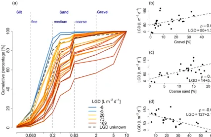
Relating grain size distributions averaged over the upper metre of the lake sediment to the strength of LGD showed that low LGD rates occurred at locations dominated by fine sand and stronger LGD rates occurred at locations with a higher fraction of larger grain sizes (Fig. 8a). LGD was pos-itively correlated with the percentage of gravel and coarse sand and negatively correlated with the percentage of fine sand (Table 3, Fig. 8b–c), but LGD rates were uncorre-lated with the grain size fractions of medium sand and silt (Table 3). LGD varied by a factor of 3 across these grain size fractions. For the multiple regression model, consider-ing all grain sizes, only coarse sand and fine sand were sig-nificant variables (pvalues<0.05). The model had an R2 of 0.54 (Table 3). The absolute residuals were on average 21 L m−2d−1, with largest positive residuals (observed less than calculated) at distances of 50 and 10 m from the north-ern tip at the eastnorth-ern and westnorth-ern shores, respectively, and largest positive residuals (observed greater than calculated) at distances of 70 and 90 m from the northern tip at the east-ern shore (Fig. 9a).
3.2.2 Topographic indices as controls on large-scale LGD patterns
Subcatchments derived from the 46 shoreline sections dif-fered significantly in size. While subcatchments in the flatter areas of the south were larger, elevations were higher and slopes generally steeper in the north. There was no clear cor-relation between LGD rates and the size of the subcatchment in each topographical zone of influence (Table 4). Percent-ages of area with low topographic gradient in direct vicinity of the lake shore area were also not correlated with LGD rates, except for zi25 m, where a weak negative correlation
[image:10.612.83.252.293.442.2]Figure 6.Lake sediment temperatures measured with the FO-DTS system.(a)Temperatures measured in February and August along the FO-DTS cable.(b)Sediment temperatures measured with the FO-DTS in August 2014 (median); LGD rates along the shoreline were derived from VTPs measured in June 2012.
Figure 7.LGD plotted against ksatvalues determined from slug tests at the western and eastern shores; the grey shading indicates the
distances of measurement locations from the northern tip of the lake.
Table 3.Correlation coefficients (ρ), linear models describing the correlation between LGD and predictors and the coefficient of de-termination (R2).ρ values given in boldface indicate significant correlation (pvalue>0.05); normal typeface values indicate in-significant correlations (pvalue<0.05).
Predictor (x) ρ Models (LGD=. . .) R2
Gravel 0.61 49.84+1.78x 0.25 Coarse sand 0.62 14.03+5.27x 0.46
Medium sand 0.01 – –
Fine sand −0.7 127–2.12x 0.48
Silt 0.01 – –
Coarse plus fine sand 72.72+3.06x1−1.35x2 0.54
[image:11.612.117.483.272.419.2]the indices’ elevation and slope were both positive (Table 4, Fig. 10b and c) and the strength of correlation was strongest for zi50 m and decreased with increasing zone of influence
(Table 4).
3.2.3 Groundwater flow field as control on large-scale LGD patterns
The water table ratio (Haitjema and Mitchell-Bruker, 2005) as an indicator for either recharge- or topography-controlled groundwater tables was determined based on conservative estimates of the input variables: annual recharge rate R=
0.00351 m d−1(based on values from Müller et al., 2009 de-termined in the same region), mean distance to the next sur-face watersLbeing approximately 2000 m,m=8 (–) for 1-D flow (however, changing this to 16 for radial flow does not change the outcome), the average hydraulic conductiv-ityk=7.776 m d−1(based on laboratory analyses of
undis-turbed cores obtained during observation well installation), average aquifer thicknessH=15 m (from bore logs) and the maximum terrain rised=52 m. The water table ratio in this case amounts to 0.029 which is1 and thus indicates that water tables in the study area are not topography controlled but instead recharge controlled.
[image:11.612.46.289.537.625.2]to-Figure 8. (a)Grain size distributions averaged over the upper metre of the lake sediment from sediment cores coloured by the strength of LGD rate; LGD rates are plotted against the grain sizes for gravel(b), coarse sand(c)and fine sand(d).
Figure 9.Observed and calculated LGD distribution along the shoreline.(a)Small-scale patterns predicted using a multiple regression model with coarse sand and fine sand as predictors and(b)large-scale patterns predicted by the linear model based on groundwater gradients derived from regression kriging from zone zi25 m. Regression equations for both small- and large-scale patterns are included in the upper right corner.
In the small-scale variability equation,x1stands for the fraction of coarse sand andx2for fine sand.
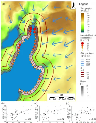
wards Lake Hinnensee from all directions (Fig. 10). In gen-eral, groundwater gradients were stronger in the north than in the south.
The maximum deviation between interpolated and mea-sured groundwater levels was below 1 cm for both interpola-tions, but in comparison to the ordinary kriging, the regres-sion kriging (which included topographical information)
re-sulted in significantly stronger gradients: median groundwa-ter gradient in the zi200 m, for example, was 0.24 cm m−1
[image:12.612.70.526.390.552.2]de-Figure 10.Correlation between far-field conditions and LGD.(a)LGD of lake subsections and mean slope of upslope areas for topographical zone of influence (zi) of 50 m; groundwater gradients (GW gradients) are derived from interpolation of measured groundwater levels using regression kriging.(b–d)LGD rates of lake subsections are plotted against the far-field conditions’ mean elevation(b), mean slope(c)and mean groundwater gradients derived from regression kriging(d)calculated for zi50 m.
Table 4.Correlation coefficients (ρ) between LGD and far-field predictors calculated for upslope areas in certain topographical zones of influence (zi).ρvalues in italic indicate insignificant coefficients (pvalue>0.05).ρvalues in bold indicate strong significant coefficients (pvalue<0.05). gg is the abbreviation for groundwater gradients and ltg the abbreviation for low topographic gradient in direct proximity to the lake shore.
Predictors/zi Size Mean elevation Mean slope Percentage of ltg Mean gg Mean gg (ordinary kriging) (regression kriging)
25 m 0.15 0.61 0.58 −0.44 0.33 0.64
50 m 0.03 0.62 0.64 −0.30 0.36 0.65
100 m −0.19 0.45 0.58 0.00 0.32 0.59
[image:13.612.75.524.617.696.2]rived from regression kriging (between 0.55 and 0.64) (Ta-ble 2). The linear predictor function used for the regression kriging was gw=62.5+0.02ewhere gw is the groundwater level in metres andethe smoothed surface elevation in me-tres. The topography was a significant model predictor with apvalue of 10−5.
3.2.4 Linear regression models between LGD and far-field predictors
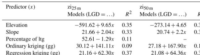
The linear regression models describing the correlation be-tween LGD and far-field conditions were estimated for all predictors of zi25 mand zi50 m. Significant predictors of LGD
large-scale patterns were elevation, slope, percentage of area with low topographic gradient (only in zi25 m) and
groundwa-ter gradients (Table 5). No significant linear regression model was found with the potential predictors “potential size of sub-catchment” and “percentage of area with low topographic gradient” in zi50 m. The R2 values of all models were not
larger than 0.37 (Table 5) but were below 0.12 for the “per-centage of area with low topographic gradient” and “ground-water gradients derived from ordinary kriging” predictors (Table 5). Therefore, these predictors were excluded for fur-ther analyses.
The calculation of multiple regression models revealed no significant relations between LGD and topographic indices in both zones of influence. Stepwise reduction of the most insignificant predictor until all predictors became significant resulted in the single linear regression models as presented above and in Table 5.
Calculated large-scale LGD patterns along the shoreline using the best linear regression model (based on groundwa-ter gradients derived from regression kriging in zi25 m;
Ta-ble 5) are shown in Fig. 9b. The general spatial pattern was captured by the model, but absolute deviations were on av-erage 10.4 L m−2d−1. Strongest overestimations occurred at distances of 500 m at the eastern and 300 m at the western shore and strongest underestimation by the model were found at distances of 450 and 150 m at the western shore.
4 Discussion
4.1 LGD patterns along the shoreline and potential controls
The experimental design based on extensive field campaigns employed here provided exceptionally detailed information on both small-scale variabilities and large-scale patterns of LGD rates along a lake shoreline. This data set thus bridges the gap between the detailed local and low-resolution larger-scale investigations of previous LGD studies.
While the employed method of measuring VTPs with a needle thermistor is sufficiently rapid to make this large high-resolution data set possible, it nevertheless takes con-siderable effort. We therefore investigated if measuring
tem-perature at just a single depth instead of measuring an en-tire depth profile (thus reducing measurement time even fur-ther) would already supply at least qualitative information on LGD patterns. We found that temperatures measured at depths larger than 20 cm generally correlated well with LGD rates, thus reproducing the general pattern of groundwater in-flow. However, to convert these temperatures to LGD rates it would be necessary to measure at least some complete pro-files for a large enough range of LGD rates to obtain a de-cent calibration. As sediment temperatures and their gradi-ents change over time, this calibration needs to be repeated at each survey date.
4.1.1 Large-scale patterns
As expected, the observed large-scale patterns of LGD at Lake Hinnensee correlated with mean groundwater gra-dients. Interestingly, even though the system classifies as recharge controlled and not topography controlled accord-ing to the water table ratio (Haitjema and Mitchell-Bruker, 2005; Gleeson et al., 2011), correlation was stronger be-tween LGD and groundwater gradients derived from regres-sion kriging (which includes topographic information) than between LGD and groundwater gradients derived from or-dinary kriging. This suggests that the groundwater surface was more realistically interpolated using regression krig-ing and indicates at least some influence of topography on groundwater movement, which is consistent with the the-ory of topography-controlled groundwater flow described by Toth (1963). The predictors based on surface slopes and sur-face elevation, hence purely topographical information, also correlated with LGD rates (with a correlation coefficient of 0.6) – another indication of at least some topographic control on the groundwater flow field. However, even the best regres-sion model (based on the groundwater table gradients from regression kriging) did not capture all of the observed vari-ability in LGD, thus suggesting the existence of additional controls. In contrast to observations of streamflow generation in mountain catchments (Jencso et al., 2009, 2010), no posi-tive correlation was found between the size of the subment and LGD rates (Table 4), indicating that surface catch-ments derived for lake subsections were not a good estimator for the amount of subsurface water flowing into the corre-sponding lake sections. We assume our result indicates that subsurface catchments differ from surface catchments which is not unusual in lowland areas. The weak negative correla-tion between LGD and the topographic index “percentage of area with low topographic gradient in direct vicinity of the lake shore” in zi25 mindicated that low topographic gradients
at the shoreline could buffer groundwater flow towards the lake.
re-Table 5.Linear regression models describing the correlation between LGD and far-field predictors and the coefficient of determination (R2). gg is the abbreviation for groundwater gradients and ltg the abbreviation for low topographic gradient in direct proximity to the lake shore.
Predictor (x) zi25 m zi50 m
Models (LGD=. . .) R2 Models (LGD=. . .) R2
Elevation −591.62+9.65x 0.35 −273.14+4.65 0.34 Slope 21.66+2.04x 0.33 20.74+2.2x 0.32
Percentage of ltg 52.61−1.29x 0.11 – –
Ordinary kriging (gg) 30.12+141.11x 0.09 27.18+167.90x 0.12 Regression kriging (gg) 21.16+62.30x 0.37 21.08+64.36x 0.36
versal are unclear. However, the neighbouring stretches of shoreline were characterized by very low LGD rates (Fig. 2), even thoughksatvalues at this section were comparably high
(Fig. 7), and thus we assume that very low hydraulic gradi-ents are the cause for the low LGD rates. While transpiration is likely to cause diurnal fluctuations in groundwater levels all around the lake, it can result in a temporary local inversion of the groundwater–lake gradients at locations where these gradients are very low (Winter et al., 1998). This could be a potential explanation for the negative LGD rates measured at this location.
4.1.2 Small-scale patterns
Our measurements revealed strong small-scale spatial vari-ability in LGD along the shoreline (Fig. 2). Absolute amounts and spatial variability of LGD were within the range of previous studies (Rosenberry et al., 2015; Blume et al.; 2013; Neumann et al., 2013). Measuring VTPs with a high measurement resolution along large parts of the shoreline highlighted furthermore that the strength of small-scale vari-ability also varies along the shoreline. This type of informa-tion is likely to be overlooked in studies focusing either on entire lake systems but using a low spatial resolution (Schnei-der et al., 2005; Meinikmann et al., 2013; Shaw et al., 2013) or using a high spatial resolution but only on a very lo-cal slo-cale (Kishel and Gerla, 2002; Blume et al.; 2013; Se-bok et al., 2013). The repetitions of VTP measurements re-vealed that the observed patterns were stable in time and are thus likely controlled by static characteristics. Differences in LGD rates measured in different years are likely the result of annual differences in groundwater recharge and thus gradi-ents of the flow field.
Surprisingly, no positive correlation was found between LGD rates and ksat values derived from slug tests at Lake
Hinnensee. The relationship betweenksatand LGD could be
confounded as a result of strong differences in hydraulic gra-dients. However, even when only adjacent measurement lo-cations with similar gradients were taken into account, no clear positive correlations appeared (Fig. 7). Slug tests were found to be the most accurate method to determineksatvalues
of sandy stream beds (Landon et al., 2001), but estimation of hydraulic conductivity is always subject to high
uncertain-ties (Landon et al., 2001; Kalbus et al., 2006). Even though the slug tests were carried out carefully, we cannot exclude that pore structure was altered during the piezometer installa-tion, and thus theksatvalues of lake sediments were changed.
In contrast toksatvalues, LGD rates clearly correlated with
both the finest and the coarsest grain size fractions. Grain sizes give no direct information on hydraulic conductivity, but coarse sand and gravel are associated with higher hy-draulic conductivity values than well-sorted fine sand (Bear, 1972). As LGD rates correlated positively with percentages of gravel and coarse sand and negatively with the percentage of fine sand, this corroborated the assumption that sediment heterogeneities do at least partially control small-scale vari-ability in LGD. We furthermore see that a variation of LGD of up to a factor of 3 can be due to grain size variability alone.
4.2 LGD patterns with increasing distance to the shore and their potential controls
[image:15.612.136.460.99.188.2]4.3 Offshore-LGD patterns and potential controls We investigated the presence and absence of offshore LGD with two natural tracers (radon and heat), and the two meth-ods led to similar results (for the radon results and discus-sion, see Appendix A). The FO-DTS measurements showed no shifts in sediment temperatures towards the groundwa-ter temperature in the flatgroundwa-ter and deeper parts of the lake (Fig. 6b), and we assume that groundwater inflow is insignif-icant here. Low radon activities measured offshore at the lake bottom across the entire lake also support this assump-tion (see Appendix A). Insignificant groundwater inflow in the flatter and deeper part of the lake is in correspondence with the theory of exponentially decreasing groundwater in-flow with distance from the shore introduced by McBride and Pfannkuch (1975). Furthermore, we know from obser-vations by divers that the lake bottom was covered with fine-grained organic sediments, which typically accumulate in the deep, flat parts, where wave action cannot resuspend the fine sediments (Rosenberry et al., 2015). A layer of fine-grained sediment could significantly decrease hydraulic conductiv-ity of the lake bed sediment and can even totally prevent groundwater–lake exchange (Kidmose et al., 2013).
FO-DTS showed local hotspots of groundwater inflow at three locations, all on steep steps between the near-shore part and the flatter central basin. These locations with sediment temperature anomalies coincided with high near-shore LGD rates (estimated with VTPs), while corners where no temper-ature anomalies were found coincided with low near-shore LGD rates (Fig. 6b). As hotspots in near-shore LGD occurred locally and mainly in the northern part of the lake, we as-sume that the occurrence of hotspots of LGD at steep steps is also a local phenomenon limited to the northern part. As the occurrence of the local sediment temperature anomalies is temporally stable (Fig. 6a), we assume that static char-acteristics are responsible – at these locations, where near-shore LGD was already strong, the morphology of steep steps might force a local offshore increase of LGD: at steep slopes, fine sediment is prone to be re-disturbed by turbidity cur-rent activities (Håkanson, 1977), locally increasing hydraulic conductivity and thus also LGD.
4.4 Prediction of LGD patterns
Using linear regression models based on topographic charac-teristics or the groundwater flow field to predict large-scale patterns of LGD at Lake Hinnensee roughly reproduced the observed patterns but locally strongly over- or underesti-mated the observed LGD rates (Fig. 9b). However, regres-sion models considering sediment heterogeneities were able to explain more than 50 % of the observed small-scale vari-ability in LGD (R2=0.55). We calculated linear regression models separately for topographic indices and sediment het-erogeneities, because sediment cores were only taken from a fraction of the lake, covering not more than one lake
sub-section used for far-field analysis. But as LGD is driven by both the hydraulic gradients between lake and aquifer and the hydraulic conductivity, combining the information would likely explain more of the observed variability. Another pos-sible influence is currently unknown local heterogeneous fea-tures within the adjoining aquifer (Winter, 1999; Cherkauer and Nader, 1989; Fleckenstein et al., 2009). Such small-scale structures may influence the groundwater flow paths and cause variability in LGD.
5 Summary and conclusion
derived from regression kriging, which also included topo-graphic information. The explanatory power of these indices was strongest when derived locally up to a distance of 50 m from the shoreline, and decreased with increasing distance from the lake. Small-scale LGD patterns in the north were linked to sediment heterogeneities: LGD patterns correlated positively with percentages of gravel and coarse sand and negatively with the percentage of fine sand. However, LGD patterns did not correlate withksatvalues derived from slug
tests. We assume that our findings are transferrable to simi-lar lowland landscapes with quasi-homogeneous aquifers. As the water table ratio at this site indicated recharge control, we assume topography to have an even greater influence on LGD patterns in areas where groundwater tables are classified as topography controlled. However, more complex hydrogeo-logical settings which include discontinuities can override and mask the topographic signal.
Our results furthermore showed that predictions of LGD rates using regression models derived from correlation with external controls were associated with high uncertainties but nevertheless allowed a rough estimation of LGD patterns. To-pographic indices, such as elevation or slope, are often read-ily available. Analysing grain size distributions of lake sedi-ment is labour intensive, but sedisedi-ment cores taken with trans-parent sampling tubes can be easily analysed at least quali-tatively. This information combined with information of to-pographic gradients can then be used to develop an effective and efficient measurement design for more a detailed char-acterization of spatial patterns of LGD that goes beyond the rough estimate that the linear regression models can provide. Measuring VTPs with a 45 cm long needle thermome-ter is a fast and inexpensive method to dethermome-termine LGD rates without disturbing the sediment. Correlation between LGD rates and temperature values measured at 30 cm depth also show that even single depth temperature measurements can provide at least some rough qualitative information on LGD patterns. While installing a fibre-optic cable along the shoreline would have the advantage of providing a large high-resolution spatial data set as well as continuous mea-surements, the cable would need to be installed at a fixed depth>20 cm to provide reliable data, uninfluenced by so-lar radiation and boundary effects. Such an installation of a kilometre-long cable at a fixed depth is challenging and would significantly disturb the sediment, potentially causing preferential flow paths and changing the very fluxes we want to measure. We therefore favour the manual measurements using the thermistor needle, as this method has furthermore the added advantage of providing temperature profiles and thus enabling us to obtain reliable quantitative estimates of LGD rates at a large number of locations.
From the experience gained in this study, we would sug-gest the following protocol for future studies of LGD patterns and controls:
1. Determine topographic indices for the 50 m region around the lake (broken down in partially overlapping subsections of a length representative of the variability in topography – in our study 100 m with 50 m overlap) and combine this with groundwater flow field informa-tion from observainforma-tion wells. Determine if system clas-sifies as groundwater or topography controlled by using the water table ratio, if only limited well information exists, to get a better idea of the groundwater table char-acteristics.
2. Predict LGD patterns based on this information. 3. Test predictions at eight locations (more if feasible) by
measuring VTPs and estimating LGD rates based on the heat transport equation. If possible, perform additional single depth temperature measurements and compare the obtained qualitative LGD patterns with the ones pre-dicted from topographic indices to further evaluate the reliability of the prediction.
4. Characterize small-scale variability at two of these lo-cations (covering high and low inflow regions) by addi-tional measurements at higher spatial resolution. 5. Use clear plastic tubes to sample sediment cores for
quick visual inspection and rough classification accord-ing to grain size/permeability and relate this to the cor-responding LGD at each of these locations.
6. If interested in the temporal stability of the LGD pat-terns, repeat step 3 at different points in time.
Appendix A: Identification of offshore lacustrine groundwater discharge based on radon concentrations
A1 Background
Radon (222Rn) is produced within the natural decay chain of uranium and has a half-life of 3.82 days. Radon occurs nat-urally in the aquifer matrix and, as it is soluble, groundwa-ter is enriched in radon as it passes through the aquifer ma-trix. However, once radon-enriched groundwater is in con-tact with air, radon degasses quickly. Consequently, radon activities in surface water are low. Due to the pronounced differences between groundwater and surface water concen-trations, elevated radon activities can be used as an indicator for groundwater inflows as shown, for example, by Kluge et al. (2012), Ono et al. (2012) and Shaw et al. (2013).
A2 Method
In this study, we used radon as a qualitative indicator of presence or absence of offshore LGD. We took water sam-ples of 1.5 or 1.75 L from the bottom of the lake (lower end of the water column) at 19 locations (Fig. A1a) during three campaigns: 5 June 2013 (seven southernmost samples), 17 September 2013 (eight samples) and 21 August 2014 (three samples along the FO-DTS cable close to corner 2; Fig. A1b). Water samples taken at along the cable were taken by divers. All other samples were taken from a boat us-ing a peristaltic pump. Contact between water samples and air was minimized and bottles were filled without air bub-bles. To test the reliability of radon concentrations to iden-tify groundwater inflow at Lake Hinnensee, we took wa-ter samples from two near-shore VTP locations where LGD rates were known and significantly different: one with strong inflow (153 L m−2d−1, located 40 m south from the north-ernmost VTP measurement location at the eastern shore; Fig. A1b) and one with medium inflow (48 L m−2d−1, lo-cated 60 m south from the northernmost VTP measurement location at the eastern shore; Fig. A1b). In order to estimate the radon activity of the groundwater, a groundwater sample was taken in a nearby piezometer (Fig. 1c of the paper). The water samples were analysed using the alpha spectrometer RAD7 (Durridge Company Inc., Bedford, MA, USA) with the Big Bottle RAD H2O extension. Analysing time of the
RAD7 was extended to 3.5 h or longer to reduce measure-ment uncertainties. To remove background concentration of radon in the measurement device, the device was purged for at least 3.5 h with fresh air between water samples. Relative humidity was kept below 8 % during measurements. Most of the samples were analysed in the first days directly after sam-pling. Maximum delay between sampling and analysis was 1 week. The data were decay corrected based on the time between sampling and analysis.
A3 Results
To test the capability of radon as a tracer of ground-water inflow at Lake Hinnensee, we took two samples at VTP measurement locations where LGD rates were known to be significantly different. The radon activity at the sampling location with stronger LGD was significantly higher (787 Bq m−3) than the radon activity in the other sample (90 Bq m−3). Groundwater had a radon activity of 12 151 Bq m−3. Radon activities in lake water samples taken offshore ranged between 0 and 103 Bq m−3, with a median of 41 Bq m−3and an IQR of 30 Bq m−3. Radon activities in the uppermost quartile (>54 Bq m−3) were measured in the northern part of the lake and at one sampling point in the central part of the lake 100 m east of the southern tempera-ture logger chain. The three southernmost points had lowest radon activities (0–22 Bq m−3) (Fig. A1).
A4 Discussion
Author contributions. CT and TB designed the experiments, dis-cussed results and wrote the paper together. CT carried out the field measurements and the data analysis.
Competing interests. The authors declare that they have no conflict of interest.
Acknowledgements. This study is a contribution to the Virtual Institute of Integrated Climate and Landscape Evolution Analysis – ICLEA – of the Helmholtz Association. We would like to thank Lisei Köhn, Christian Budach, Sigfried Tusche, Philip Müller, Markus Morgner, Henriette Wilke and Knut Günther for their help in the field, the divers Silke Oldorff and Frank Kroll for their help laying out the FO-DTS cable and the Mueritz National Park authorities for their cooperation. Furthermore we thank Matthias Munz and Jana Carus for helpful discussions in the early stage of the manuscript. Bathymetry data were provided by the Ministerium für Landwirtschaft, Umwelt und Verbraucherschutz Mecklenburg-Vorpommern. The study took place in the TERENO observatory of north-east Germany funded by the Helmholtz Association. We thank the anonymous reviewers for their very helpful comments that greatly improved the manuscript.
The article processing charges for this open-access publication were covered by a Research
Centre of the Helmholtz Association.
Edited by: Thom Bogaard
Reviewed by: three anonymous referees
References
Bear, J.: Dynamics of fluids in porous media, Elsevier, New York, 1972.
Blume, T., Krause, S., Meinikmann, K., and Lewandowski, J.: Upscaling lacustrine groundwater discharge rates by fiber-optic distributed temperature sensing, Water Resour. Res., 49, 7929– 7944, https://doi.org/10.1002/2012wr013215, 2013.
Born, S. M., Smith, S. A., and Stephenson, D. A.: Hydrogeol-ogy of glacial-terrain lakes, with management and planning ap-plications, J. Hydrol., 43, 7–43, https://doi.org/10.1016/0022-1694(79)90163-x, 1979.
Bredehoeft, J. D. and Papaopulos, I. S.: Rates of verti-cal groundwater movement estimated from the Earth’s thermal profile, Water Resour. Res., 1, 325–328, https://doi.org/10.1029/WR001i002p00325, 1965.
Brenning, A.: Statistical Geocomputing combining R and SAGA: The Example of Landslide susceptibility Analysis with general-ized additive Models, in: SAGA – Seconds Out, edited by: Böh-ner, J., Blaschke, T., and Montanarella, L., Hamburger Beiträge zur Physischen Geographie und Landschaftsökologie, 19, 23–32, 2008.
Brock, T. D., Lee, D., Janes, D., and Winek, D.: Ground-water seepage as a nutrient source to a drainage lake, Lake Mendota, Wisconsin, Water Res., 16, 1255–1263, https://doi.org/10.1016/0043-1354(82)90144-0, 1982.
Caruso, A., Ridolfi, L., and Boano, F.: Impact of watershed topog-raphy on hyporheic exchange, Adv. Water Resour., 94, 400–411, https://doi.org/10.1016/j.advwatres.2016.06.005, 2016. Chapuis, R. P.: Shape factors for permeability tests in
bore-holes and piezometers, Ground Water, 27, 647–654, https://doi.org/10.1111/j.1745-6584.1989.tb00478.x, 1989. Cherkauer, D. S. and Nader, D. C.: Distribution of
ground-water seepage to large surface-ground-water bodies: the effect of hydraulic heterogeneities, J. Hydrol., 109, 151–165, https://doi.org/10.1016/0022-1694(89)90012-7, 1989.
Fleckenstein, J. H., Neumann, C., Volze, N., and Beer, J.: Raumzeitmuster des See-Grundwasser-Austausches in einem sauren Tagebaurestsee, Grundwasser, 14, 207–217, https://doi.org/10.1007/s00767-009-0113-1, 2009.
Gleeson, T., Marklund, L., Smith, L., and Manning, A. H.: Classi-fying the water table at regional to continental scales, Geophys. Res. Lett., 38, L05401, https://doi.org/10.1029/2010GL046427, 2011.
Grimm, V., Revilla, E., Berger, U., Jeltsch, F., Mooij, W. M., Rails-back, S. F., Thulke, H.-H., Weiner, J., Wiegand, T., and DeAn-gelis, D. L.: Pattern-oriented modeling of agent-based com-plex systems: lessons from ecology, Science, 310, 987–991, https://doi.org/10.1126/science.1116681, 2005.
Haitjema, H. M. and Mitchell-Bruker, S.: Are water tables a sub-dued replica of the topography?, Groundwater, 43, 781–786, 2005.
Håkanson, L.: The influence of wind, fetch, and water depth on the distribution of sediments in Lake Vänern, Sweden, Can. J. Earth Sci., 14, 397–412, https://doi.org/10.1139/e77-040, 1977. Hvorslev, M. J.: Time lag and soil permeability in ground-water
observations, US Army Corps of Engineers, Vicksburg, Missis-sippi, Waterways Experiment Station Bulletin, 36, 1–50, 1951. Jencso, K. G., McGlynn, B. L., Gooseff, M. N., Wondzell, S. M.,
Bencala, K. E., and Marshall, L. A.: Hydrologic connectivity be-tween landscapes and streams: transferring reach- and plot-scale understanding to the catchment scale, Water Resour. Res., 45, W04428, https://doi.org/10.1029/2008wr007225, 2009. Jencso, K. G., McGlynn, B. L., Gooseff, M. N., Bencala, K. E.,
and Wondzell, S. M.: Hillslope hydrologic connectivity controls riparian groundwater turnover: implications of catchment struc-ture for riparian buffering and stream water sources, Water Re-sour. Res., 46, W10524, https://doi.org/10.1029/2009wr008818, 2010.
Kalbus, E., Reinstorf, F., and Schirmer, M.: Measuring methods for groundwater – surface water interactions: a review, Hydrol. Earth Syst. Sci., 10, 873–887, https://doi.org/10.5194/hess-10-873-2006, 2006.
Kidmose, J., Nilsson, B., Engesgaard, P., Frandsen, M., Karan, S., Landkildehus, F., Søndergaard, M., and Jeppesen, E.: Focused groundwater discharge of phosphorus to a eutrophic seep-age lake (Lake Væng, Denmark): implications for lake eco-logical state and restoration, Hydrogeol. J., 21, 1787–1802, https://doi.org/10.1007/s10040-013-1043-7, 2013.
Kishel, H. F. and Gerla, P. J.: Characteristics of preferential flow and groundwater discharge to Shingobee Lake, Minnesota, USA, Hy-drol. Process., 16, 1921–1934, https://doi.org/10.1002/hyp.363, 2002.