Towards a simple representation of chalk hydrology in land surface modelling

www.hydrol-earth-syst-sci.net/21/459/2017/ doi:10.5194/hess-21-459-2017

© Author(s) 2017. CC Attribution 3.0 License.

Towards a simple representation of chalk hydrology

in land surface modelling

Mostaquimur Rahman1and Rafael Rosolem1,2

1_{Department of Civil Engineering, University of Bristol, Bristol, UK} 2_{Cabot Institute, University of Bristol, Bristol, UK}

Correspondence to:Mostaquimur Rahman ([email protected])

Received: 18 May 2016 – Published in Hydrol. Earth Syst. Sci. Discuss.: 26 May 2016 Revised: 7 January 2017 – Accepted: 9 January 2017 – Published: 25 January 2017

Abstract. Modelling and monitoring of hydrological pro-cesses in the unsaturated zone of chalk, a porous medium with fractures, is important to optimize water resource as-sessment and management practices in the United King-dom (UK). However, incorporating the processes governing water movement through a chalk unsaturated zone in a nu-merical model is complicated mainly due to the fractured nature of chalk that creates high-velocity preferential flow paths in the subsurface. In general, flow through a chalk un-saturated zone is simulated using the dual-porosity concept, which often involves calibration of a relatively large number of model parameters, potentially undermining applications to large regions. In this study, a simplified parameterization, namely the Bulk Conductivity (BC) model, is proposed for simulating hydrology in a chalk unsaturated zone. This new parameterization introduces only two additional parameters (namely the macroporosity factor and the soil wetness thresh-old parameter for fracture flow activation) and uses the satu-rated hydraulic conductivity from the chalk matrix. The BC model is implemented in the Joint UK Land Environment Simulator (JULES) and applied to a study area encompass-ing the Kennet catchment in the southern UK. This param-eterization is further calibrated at the point scale using soil moisture profile observations. The performance of the cali-brated BC model in JULES is assessed and compared against the performance of both the default JULES parameterization and the uncalibrated version of the BC model implemented in JULES. Finally, the model performance at the catchment scale is evaluated against independent data sets (e.g. runoff and latent heat flux). The results demonstrate that the inclu-sion of the BC model in JULES improves simulated land surface mass and energy fluxes over the chalk-dominated

Kennet catchment. Therefore, the simple approach described in this study may be used to incorporate the flow processes through a chalk unsaturated zone in large-scale land surface modelling applications.

1 Introduction

Chalk can be described as a fine-grained porous medium traversed by fractures (Price et al., 1993). Previous studies showed that the unsaturated zone of the chalk aquifers plays an important role in groundwater recharge in the UK (e.g. Lee et al., 2006; Ireson et al., 2009). Therefore, both moni-toring (e.g. Bloomfield, 1997; Ireson et al., 2006) and mod-elling (e.g. Bakopoulou, 2015; Brouyère, 2006; Ireson and Butler, 2011, 2013; Sorensen et al., 2014) strategies have been adapted previously to understand the governing hydro-logical processes in the chalk unsaturated zone.

In chalk, the matrix provides porosity and storage capac-ity, while the fractures greatly enhance permeability (Van den Daele et al., 2007). Water movement through the chalk ma-trix is slow due to its relatively high porosity (0.3–0.4) and low permeability (10−9–10−8m s−1). A fractured chalk sys-tem, in contrast, conducts water at a considerably higher velocity because of the relatively high permeability (10−5_–

10−3m s−1) and low porosity (of the order 10−4) of fractures (Price et al., 1993).

flow through the chalk unsaturated zone. The physics-based models mentioned above were developed based on a dual-continua approach and required relatively large numbers of parameters (i.e. of the order of 20–30 parameters) that were calibrated via inverse modelling using observed soil moisture and matric potential data (e.g. Ireson et al., 2009; Mathias et al., 2006).

In recent years, representation of chalk has gained at-tention in land surface modelling. For example, Gas-coin et al. (2009) applied the Catchment Land Surface Model (CLSM) over the Somme River basin in northern France. A linear reservoir was included in the TOPMODEL-based runoff formulation of the CLSM to account for the contribution of chalk aquifers to river discharge. Le Vine et al. (2016) applied the Joint UK Land Environment Sim-ulator (JULES; Best et al., 2011) over the Kennet catch-ment in southern England to evaluate the hydrological limi-tations of land surface models. In that study, two intersecting Brooks and Corey curves were proposed, which allowed a dual-curve soil moisture retention representation for the two distinct flow domains of chalk (i.e. matrix and fracture) in the model. Considering this dual Brooks and Corey curve, a three-dimensional groundwater flow model (ZOOMQ3D; Jackson and Spink, 2004) was coupled to JULES to demon-strate the strong influence of representing chalk hydrology and groundwater dynamics on simulated soil moisture and runoff.

The above-mentioned studies illustrate the importance of representing chalk in land surface modelling. However, in-cluding chalk hydrology in large-scale land surface mod-elling using the contemporary dual-porosity concept can be complicated due to the large number of additional param-eters. In this context, we propose a new parameterization, namely the Bulk Conductivity (BC) model, as a first step to-wards a simple chalk representation suitable for land surface modelling. In order to test the proposed parameterization, the BC model is included in JULES (version 4.2), which, by de-fault (i.e. uniform soil column representation using a general soil database as typically applied in land surface models), does not represent any chalk feature. In this study, the BC model (included in JULES) is applied at two distinct spa-tial scales (i.e. point and catchment). At the point scale, the proposed parameterization is calibrated using observed soil moisture profile data. This is achieved by randomly sampling the parameter space and extensively running the model in or-der to minimize the differences between observed and simu-lated soil moisture variability at different depths. Finally, the proposed model is applied to the Kennet catchment in south-ern England and the fluxes and states of the hydrological cy-cle are simulated for multiple years. The simulation results are evaluated using observed latent heat flux (LE) and runoff data to assess the performance of the BC model in simulating land surface processes at the catchment scale.

2 A model of flow through a chalk unsaturated zone In this study, the BC model based on the work by Zehe et al. (2001) is incorporated into JULES to represent the flow of water through the fractured chalk unsaturated zone. Accord-ing to this approach, if the relative saturation (S) exceeds a certain threshold (S0) at a soil grid, the saturated hydraulic

conductivity of the chalk matrix (Ks) is increased to a bulk

saturated hydraulic conductivity (Ksb) as follows: Ksb=Ks+Ksfm

S−S0

1−S0

ifS > S0, (1)

Ksb=KsifS <=S0, (2)

with

S= θ−θr

θs−θr ,

wherefm is a macroporosity factor (–), θ is soil moisture

(m3m−3),θsis soil moisture at saturation (m3m−3) andθris

the residual soil moisture (m3m−3). Note thatSranges from 0 in the case of completely dry soils to 1 for fully wet soils.

At the first step of evaluation, the Ks, S0 and fm

pa-rameters are estimated based on the existing literature to assess the performance of the uncalibrated BC model. For the matrix saturated hydraulic conductivity (Ks), we use Ks=1.0 mm day−1following Mathias et al. (2006). In

addi-tion, Eq. (1) indicates that the onset of water flow through the fracture system of chalk is controlled by the thresholdS0.

Ac-cording to Wellings and Bell (1980), water flow through frac-tures dominates over matrix flow in chalk when the pressure head in soil becomes higher than−0.50 m H2O. We consider

a value ofS0=0.80 for the uncalibrated BC model, which

is based on the observed soil moisture–matric potential rela-tionship in the study area.

Finally, in Zehe et al. (2001),fmwas defined as the ratio of

the saturated water flow rate in all macropores in a model ele-ment to the corresponding value in the soil matrix, which can be determined based on the density and length of fractures on small scales. In addition,fmhas also been considered as

a calibration parameter previously (e.g. Blume, 2008; Zehe et al., 2013). In this study, we definefmas a characteristic

soil property reflecting the influence of fractures on soil wa-ter movement (Zehe and Blöschl, 2004) and estimate it from the relative difference of permeability between chalk matrix and fractured chalk system that can be of the order 104–106 according to Price et al. (1993). Consequently, we consider a macroporosity factor offm=105for the uncalibrated BC

Table 1.Field measurements and remote sensing data.

Data Spatial Temporal Frequency Source

scale extent

Soil moisture Pointa 2003–2005 15-day N. Hewitt (CEH) Latent heat flux Global 2006–2011 8-day, 1-month MODIS

Discharge Pointb 2006–2011 1-day NRFA

a_{Measured at Warren Farm;}b_{Locations are shown in Fig. 1a.}

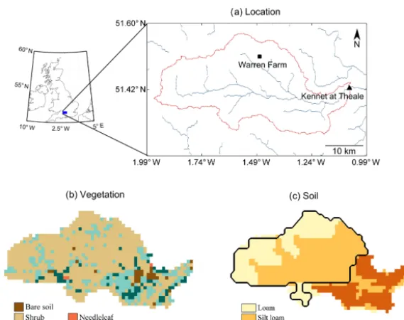
Figure 1. (a) Location,(b)vegetation cover and (c)soil texture over the study area. The red line in (a)outlines the Kennet catchment boundary, while the river network is shown in blue. The black triangle in(a)shows the location of the discharge gauging station at the catchment outlet and the black square corresponds to the Warren Farm location where point-scale simulations are carried out. The black line in(c)encloses the area of the catchment where chalk is present.

3 Methods 3.1 Study area

The study area encompasses the Kennet catchment located in southern England, with an area of about 1033 km2(Fig. 1a). Generally, Kennet is rural in nature with scattered settlements and has a maximum altitude of approximately 297 m (above ordnance level). The River Kennet discharges into the North Sea through London. The major tributaries of this river are Lambourn, Dun, Enborne, and Foudry Brook. An average annual rainfall of approximately 760 mm was recorded in the catchment over a 40-year period from 1961 to 1990.

The solid geology of the Kennet catchment is dominated by chalk, which is overlain by a thin soil layer. While lower chalk outcrops along the northern catchment boundary, pro-gressively younger rocks are found in the southern part. In general, surface runoff production is very limited over the regions of the catchment where chalk outcrops. The flow regime shows a distinct characteristic of slow response to

groundwater held within the chalk aquifer (Le Vine et al., 2016). According to Ireson and Butler (2013), the unsatu-rated zone of chalk shows slow drainage over summer and bypass flow during wet periods in this catchment.

The National River Flow Archive (NRFA) coordinates discharge measurements from the gauging station networks across the UK. These networks are operated by the En-vironmental Agency (England), Natural Resources Wales, the Scottish Environment Protection Agency, and the Rivers Agency (Northern Ireland). We use discharge measurements provided by the NRFA to assess model performance in sim-ulating runoff over the Kennet catchment in this study.

The MOD16 product of the Moderate Resolution Imag-ing Spectroradiometer (MODIS) is a part of the NASA/EOS project that provides estimation of global terrestrial LE. The LE estimation from MOD16 is based on remotely sensed land surface data (e.g. Mu et al., 2007). In this study, the 8-day and monthly LE data products from MODIS are used to evaluate the model performance in simulating land surface energy fluxes.

3.3 Land surface model

In this study, we use the Joint UK Land Environment Sim-ulator (JULES; e.g. Best et al., 2011; Clark et al., 2011) version 4.2. JULES is a flexible modelling platform with a modular structure aligned to various physical processes de-veloped based on the Met Office Surface Exchange Scheme (MOSES; e.g. Cox et al., 1999; Essery et al., 2001). Me-teorological data including precipitation, incoming short-and long-wave radiation, temperature, specific humidity, sur-face pressure, and wind speed are required to drive JULES. Each grid box in JULES can comprise nine surface types (broadleaf trees, needleleaf trees, C3 grass, C4 grass, shrubs, inland water, bare soil, and ice) represented by respective fractional coverage. Each surface type is represented by a tile and a separate energy balance is calculated for each tile.

Subsurface heat and water transport equations are solved based on finite difference approximation in JULES as de-scribed in Cox et al. (1999). Moisture transport in the sub-surface is described by the finite difference form of Richards’ equation. The vertical soil moisture flux is calculated using Darcy’s law. While the top boundary condition to solve the Richards’ equation is infiltration at the soil surface, the bot-tom boundary condition in JULES is free drainage that con-tributes to subsurface runoff.

Surface runoff is calculated by combining the equations of throughfall and grid box average infiltration in JULES. In order to direct the generated runoff to a channel network, river routing is implemented based on the discrete approxi-mation of a one-dimensional kinematic wave equation (e.g. Bell et al., 2007). In this approach, a river network is derived from the digital elevation model (DEM) of the study area and different wave speeds are applied to surface and subsurface runoff components and channel flows (e.g. Bell and Moore, 1998). A return flow term accounts for the transfer of wa-ter between subsurface and land surface (e.g. Dadson et al., 2010, 2011).

3.4 Model configurations and input data

In this study, simulations are performed at two distinct spa-tial scales, namely point and catchment. At the point scale, JULES is configured to simulate the mass and energy fluxes at the Warren Farm site (Fig. 1a). A total subsurface depth of 5 m is considered in the model with a vertical discretization ranging from 10 cm at the land surface to 50 cm at the bottom of the model domain. Note that this discretization is consis-tent with the soil moisture measurement depths mentioned in Sect. 3.2. The vegetation type is implemented as C3 grass using the default parameters in JULES. Point-scale simula-tions were performed over 2 consecutive years from 2003 to 2005 at an hourly time step. Except for precipitation, hourly atmospheric forcing data to drive JULES were obtained from an automatic weather station operated by the CEH at Warren Farm. In order to estimate hourly precipitation data to run JULES, rain gauge measurements from the Met Office (Met Office, 2006) were used. The inverse distance interpolation technique (e.g. Garcia et al., 2008; Ly et al., 2013) was ap-plied to rainfall measurements from the 13 gauges closest to Warren Farm (the distance varies from 25 to 60 km) to obtain hourly precipitation for the point-scale simulations.

At the catchment scale, JULES is configured over a study area encompassing the Kennet catchment (Fig. 1a) considering a uniform lateral grid resolution of 1 km with 70×40 cells in thexandydimensions, respectively. The to-tal subsurface depth and vertical discretization are identical to those of the point-scale simulations. Spatially distributed vegetation-type information for the study area (Fig. 1b) is obtained from the Land Cover Map 2007 (LCM2007) data set (Morton et al., 2011). Simulations were performed over 5 consecutive years from 2006 to 2011 at the catchment scale. Note that the simulation periods of catchment and point scale (2003–2005) do not coincide due to the avail-ability of soil moisture measurements described in Sect. 3.2. Spatially distributed meteorological data from the Climate, Hydrology and Ecology research Support System (CHESS) were used to obtain the atmospheric forcing to drive JULES at the catchment scale. The CHESS data include 1 km resolu-tion gridded daily meteorological variables (Robinson et al., 2015). These daily data are downscaled using a disaggrega-tion technique described in Williams and Clark (2014) to ob-tain hourly atmospheric forcing. The flow direction required for river routing is extracted from the USGS HydroSHEDS digital elevation data (Lehner et al., 2008).

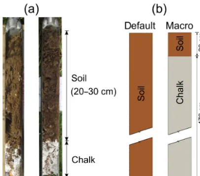
Figure 2. (a)Example of soil profiles collected at Warren Farm dur-ing a field campaign in 2015 and(b)the two model configurations.

The hydraulic properties for chalk used in this study are summarized in Table 3. These properties are obtained based on the existing literature as a first step when evaluating the uncalibrated BC model. The BC model parameters are sub-sequently calibrated to minimize the differences between ob-served and simulated1θ(Sect. 3.5) at various soil depths.

In this study, we consider two different model configura-tions, namely default and macro (Fig. 2). The default con-figuration corresponds to the standard parameterizations of JULES that does not represent chalk hydrology in the model. In this configuration, each soil column in JULES is consid-ered to be vertically homogeneous with the soil properties defined in Table 2, which is motivated by the Met Office JULES Global Land 4.0 configuration described in Walters et al. (2014). The macro configuration, in contrast, explicitly represents chalk by applying the BC model starting at 30 cm below the land surface to the bottom of the model domain (i.e. 500 cm). Therefore, the soil column in the macro con-figuration can be divided into topsoil (0–30 cm) and chalk (30–500 cm). The topsoil depth of 30 cm is defined based on several augured soil samples collected during a field cam-paign at Warren Farm in 2015 (Fig. 2). This depth is corrob-orated by additional information from the British Geological Survey (BGS) operated borehole records (http://www.ukso. org/pmm/soil_depth_samples_points.html), which show that topsoil depths vary from 10 to 40 cm over the study area. We apply the macro configuration assuming a spatially homoge-neous topsoil depth of 30 cm for both point- and catchment-scale simulations. Note that except for this inclusion of chalk, default and macro configurations are identical in terms of model set up and input data. It should also be emphasized that default represents a “naïve” configuration deprived of model calibration. Moreover, this configuration does not represent chalk, which, according to previous studies (e.g. Le Vine et

Table 2. Hydraulic properties for different soil types (refer to Fig. 1c). Saturated hydraulic conductivity (Ks) and porosity data are obtained from Rawls et al. (1982). The Van Genuchten parame-ters are acquired from Schaap and Leij (1998).

Texture Ks Porosity α n

(mm day−1) (–) (m−1) (–)

Loam 320 0.463 3.33 1.56

Silt loam 172 0.50 1.2 1.39

Clay 15 0.475 2.12 1.2

al., 2016), substantially affects the hydrology of the study area considered here.

3.5 Calibration of the BC model

We calibrate the BC model at the point scale to minimize the differences between observed and simulated soil moisture variability (1θ) at different depths. The root mean squared error (RMSE) is used as the objective function to optimize the BC model parameters (e.g. Ireson et al., 2009):

RMSE= 1

nd nd

X

1

v u u t

1

nt−1

nt

X

2

1θ_d,tobs−1θ_d,tsim2

!

, (3)

wherendis the number of soil layers,ntis the number of soil moisture observations available for a layerd,1θobsis the ob-served variability of soil moisture and1θsimis the simulated variability of soil moisture. Note that we consider 1θ for this optimization because of its relevance to the water flux and recharge through a chalk unsaturated zone (e.g. Ireson and Butler, 2011).

Equation (1) reveals that the calibration of the BC model involves optimizing three parameters, namely the saturated hydraulic conductivity of the chalk matrix (Ks), the

satura-tion threshold (S0), and the macroporosity factor (fm). Ireson

et al. (2009) suggested a range of 0.2–2.0 mm day−1forKs.

On the other hand, Price et al. (1993) argued that, in general,

Ks is around 3–5 mm day−1for most chalk soils. Therefore,

we consider a range of 0.2–5.0 mm day−1in optimizingKs.

We consider theS0range 0–1, representing the entire

phys-ical domain for soil wetness from fully dry to fully wet, re-spectively. Forfm, a range of 104–106is considered, which,

as discussed earlier, is consistent with the relative difference between the permeability of fractured chalk and chalk matrix according to Price et al. (1993). The Latin hypercube sam-pling technique (e.g. Mckay et al., 2000) is used to generate 2000 random samples for each BC model parameter within the ranges discussed above. Note that for theKs parameter,

Table 3.Hydraulic properties of chalk.

Properties Uncalibrated Range for Calibrated

Value Source calibration value

Ks(mm day−1) 1.0 Price et al. (1993) 0.2–5.0 0.31

S0(–) 0.8 Observations 0.0–1.0 0.46

fm(–) 105 Price et al. (1993) 104–106 105∗

α(m−1) 3.0 Le Vine et al. (2016) – –

n(–) 1.4 Le Vine et al. (2016) – –

∗_f

mparameter not calibrated.

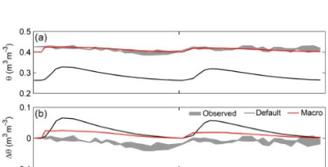
Figure 3. Comparison between observed and simulated (a)soil moisture (θ) and(b)change in soil moisture (1θ) from the default and macro configurations at a depth of 2 m below the land surface at the Warren Farm site. The shaded areas constructed from two soil moisture probes at the Warren Farm site denote the range of ob-served data in these plots.

model for each possible parameter combination as discussed in detail in the following section.

4 Results and discussion 4.1 Point-scale simulations

At the point scale, the simulation results are evaluated us-ing soil moisture observations at the Warren Farm site. Fig-ure 3a compares observed and simulated soil moistFig-ure (θ) from the default and macro configurations at 2 m below the land surface. Note that the macro configuration uses the chalk hydraulic parameters collected from the existing lit-erature (Table 3). This figure shows that the default config-uration considerably underestimatesθ throughout the simu-lation period, which is improved remarkably in the case of macro. Figure 3b plots observed and simulated soil moisture variability (1θ) from the default and macro configurations (1θdefaultand1θmacro, respectively) at the Warren Farm site.

In general, both configurations show discrepancies with ob-served1θ with macro showing relatively better model per-formance.

The results show that despite the macro configuration im-proves simulatedθ, it shows considerable discrepancies with

observed1θ, which is consistent throughout the whole chalk profile (results from other model layers are not shown). In or-der to minimize the differences between observed and mod-elled1θfrom the macro configuration, we calibrate the BC model following the methodology described in Sect. 3.5. The optimization results are summarized in Fig. 4. Note that for each combination considered in the optimization, 2000 model runs were performed using randomly sampled parameters as discussed in Sect. 3.5. In addition to the default and macro cases, the calibrated cases in Fig. 4 correspond to the results from the model runs yielding the lowest RMSE for each parameter combination evaluated.

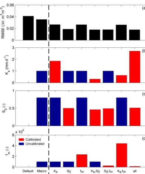
The RMSE between observed and simulated 1θ for the model configurations considered in the optimization is shown in Fig. 4a. This figure illustrates that the RMSE of the default configuration is larger than that of macro, indicating better model performance in reproducing1θ for the latter (corresponding to a reduction of 15 % in RMSE compared to the default case). Therefore, the uncalibrated BC model (i.e. macro configuration) better reproduces the soil moisture variability compared to the default. Concerning the calibra-tion of single BC model parameters, Fig. 4a shows thatS0

results in a 46 % reduction of RMSE compared to the macro configuration. CalibratingKsorfmindividually yields only

about a 25 % reduction of RMSE compared to macro. Optimizing both Ks and S0 simultaneously shows the

largest reduction (50 %) of RMSE compared to macro, which coincides with the total RMSE reduction found when all pa-rameters are calibrated. Arguably, the BC model can be im-plemented in other chalk regions by constraining only the

S0 parameter. Such a result could potentially be

advanta-geous for transferability to other regions in the UK in order to assess chalk hydrology on a large scale. However, since this is the first time the BC model is introduced, we decide to take a conservative approach and select the macro con-figuration with optimizedKsandS0(macroopthereafter) to

simulate chalk hydrology over the study area that ensures the best overall model performance.

cali-Figure 4. (a)Model performance in reproducing observed and sim-ulated1θ, (b)Ks,(c)S0and(d) fmfor the different parameter combinations considered in the optimization. For each parameter (i.e.b,c, andd), the red bars show cases in which the relevant pa-rameter is calibrated (either individually or in combination with oth-ers), while the blue bars correspond to cases in which the selected parameter is not calibrated (i.e. a fixed value according to the lit-erature as in the macro case). Note that except for the default and macro, the simulation yielding the lowest RMSE (out of 2000 model runs) is presented in this plot.

brated. The red bars in Fig. 4b–d highlight the cases in which a given parameter is constrained by optimization. In those cases, the calibrated parameter values are obtained from model runs producing the lowest RMSE. An interest-ing feature in Fig. 4b (calibratinterest-ingKsindividually) is that the

optimization suggests a compensation mechanism in which

Ks is increased remarkably in order to physically represent

the “effective” flow through the chalk fractures in the BC model. This is not surprising and arguably the simplest way to attempt to improve model performance. For macroopt, the

value used forKs is relatively lower than that of the

uncal-ibrated macro case nevertheless consistent with previous es-timates (e.g. Ireson et al., 2009). Figure 4c clearly shows the dominance of S0 in the BC model as all the relatively

low RMSE bars in Fig. 4a are associated withS0calibration

(see red bars in Fig. 4c). In addition, calibratedS0values for

all cases show a consistent constraint around 0.50. Finally, Fig. 4d indicates the lack of influence for fmparameter on

model performance.

Figure 5 compares1θdefault, 1θmacro, and 1θ from the

macroopt configuration (1θopt) with observed soil

mois-ture variability (1θobs). As mentioned earlier,1θdefault and 1θmacro show considerable discrepancies with1θobs, while

the macro configuration exhibits relatively better perfor-mance (Fig. 3). Figure 5 illustrates that the overall agreement between observed and simulated1θ improves substantially in the case of macrooptcompared to the default and macro,

which is pronounced, especially in the deeper chalk layers. Therefore, this figure indicates that the performance of the BC model in simulating1θis further improved by optimiz-ing theKs andS0 parameters simultaneously at the Warren

Farm site.

As mentioned earlier, efficiently reproducing soil mois-ture variability over the profile is important due to the fact that1θsignificantly affects water flux and recharge through the chalk unsaturated zone. The drainage flux through the bottom of the soil column (db) of a land surface model can

be considered the potential recharge flux to groundwater (e.g. Sorensen et al., 2014). Figure 6 compares the daily sum ofdb

from the default and macroopt configurations at the Warren

Farm site. Daily rainfall at this site over the simulation pe-riod is shown in Fig. 6a. In Fig. 6b, the macroopt

configura-tion shows considerabledbduring the colder months, while

relatively slow drainage is observed in summer. In contrast, the default configuration shows relatively high db in

sum-mer compared to the colder months. In general, the recharge rate through the chalk unsaturated zone during the warmer periods of the year is lower than that in the winter months (Wellings and Bell, 1980; Ireson et al., 2009). Therefore, the macroopt configuration appears to be more consistent with

the recharge mechanism in chalk compared to the default. In this section, the BC model was evaluated at the point scale. The results showed that, in general, the macro con-figuration outperforms the default case in simulating1θ. In order to improve the model performance even further, model parameter calibration was performed to minimize the differ-ences between observed and simulated1θat the point scale. In the next sections, the optimized model (macroopt) is

eval-uated at the catchment scale. 4.2 Catchment-scale simulations

At the catchment scale, simulation results from the default and macroopt configurations are compared with the

obser-vations over the Kennet catchment. In order to assess the differences between LE from the default and macroopt

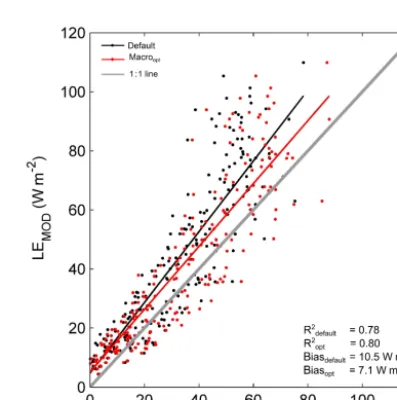
con-figurations at the catchment scale, Fig. 7 plots spatially averaged 8-day composites of LE from MODIS (LEMOD)

against the LE from these configurations (LEdefaultand LEopt,

respectively) over Kennet. The agreement between simu-lated LE and LEMOD is evaluated using the coefficient of

determination (R2; see the Appendix) and the mean bias. Comparison between LEdefault and LEMOD shows a

Figure 5.Comparison between observed and simulated1θ from default, macro and macrooptconfigurations at various depths below the land surface. The shaded areas, which are constructed from two soil moisture probes at the Warren Farm site, denote the range of1θ.

Figure 6. (a)Daily precipitation and(b)daily drainage through the bottom of the soil column at Warren Farm over the 2 simulated years (2003–2005).

biasdefault=10.5 W m−2. The agreement between simulated

LE and LEMOD improves in the case of the macroopt

con-figuration, which is reflected by an increased coefficient of determination of R2_opt=0.80 and a reduced mean bias of biasopt=7.1 W m−2.

Figure 7 shows considerable differences between LEdefault

and LEopt for relatively high LE, indicating discrepancies,

especially during the warmer months of the year. Spatially averaged time series of monthly LEMOD, LEdefault, and LEopt

are presented in Fig. 8a. This figure shows that the differ-ences between LEdefaultand LEoptincrease in summer

com-pared to the colder months of the year, which is consistent with Fig. 7. Consequently, the default configuration

under-Figure 7.Catchment average 8-day composites of MODIS esti-mated LE (LEMOD) against simulated LE from the default and macro configurations (LEdefault and LEmacro, respectively) along with the linear models fitted for LEdefault(black line) and LEmacro (red line). The 1 : 1 line is shown in grey, which represents the per-fect fit between LEMODand simulated LE.

estimates LE in summer compared to LEMOD, which is

im-proved in the case of the macrooptconfiguration. In contrast,

the differences between LEdefault and LEopt are negligible

Figure 8. (a) Spatially averaged monthly latent heat flux (LE) from MODIS, default and macroopt configurations over the Ken-net catchment and(b)monthly average observed and simulated dis-charge from the default and macrooptconfigurations at the Kennet at Theale gauging station.

In addition, Fig. 8b compares the observed and simulated monthly average discharge from the two model configura-tions at the Kennet at Theale gauging station (Fig. 1a). This figure shows that the default configuration generally over-estimates discharge at this gauging station, which is im-proved considerably in the case of macroopt. We use the

Kling–Gupta efficiency criterion (KGE; Gupta et al., 2009) to compare the performance of the two model configurations in reproducing observed discharge variability. As mentioned above, the default configuration overestimates discharge with KGEdefault= −0.17. On the other hand, the macroopt

config-uration improves the agreement between observed and simu-lated discharge, which is reflected by KGEopt=0.51.

In order to summarize the results at the catchment scale, Table 4 compares observed and simulated runoff from the two model configurations over the Kennet catchment from 2006 to 2011. The runoff ratio (RR; see the Appendix), which is equal to the mean volume of flow divided by the volume of precipitation (e.g. Kelleher et al., 2015), assesses the partitioning of precipitation into runoff over the catch-ment. The default configuration (RR=0.82) shows consid-erably higher RR compared to observation (RR=0.40), in-dicating overestimation of runoff by the model that is con-sistent with Fig. 8b. Including chalk hydrology in the model remarkably improves the agreement between observed and simulated mean runoff over the Kennet catchment, which is assessed from a runoff ratio of RR=0.46 for the macroopt

configuration, which is much closer to the observed RR value than the default.

In Table 4, the relative bias (1µ) of 1.04 between ob-served and simulated runoff from the default configuration again indicates the overestimation by the model. In compar-ison, macrooptshows a smaller relative bias of 1µ=0.12,

indicating improved agreement between observed and sim-ulated mean runoff volume compared to the default. The relative difference in standard deviation (1σ; see the

Ap-Table 4.Comparison between observed and simulated daily aver-age runoff from the two configurations over the Kennet catchment. Metrics include the runoff ratio (RR), relative bias (1µ), and rel-ative difference in standard deviation (1σ) (refer to the Appendix for further information).

Metric Observed Simulated Simulated (default) (macro)

RR 0.40 0.82 0.46

1µ – 1.04 0.12

1σ – 2.04 0.65

pendix) compares the variability of observed and simulated flow in Table 4 relating directly to the seasonal change in runoff. This comparison shows that the default configura-tion overestimates the variability of runoff over the Kennet catchment (1σ=2.04), which is improved in the case of macro (1σ=0.65). This improvement in reproducing flow variability is also clearly observed in Fig. 8b.

In this section, the BC model is evaluated using observed mass and energy fluxes over the Kennet catchment. The de-fault configuration suggested relatively low summertime LE over the catchment. The agreement between observed and simulated LE was improved in the case of the macroopt

con-figuration compared to the default. It was also observed that the overall runoff prediction was considerably improved by macroopt compared to the default. Given its simplicity, our

results indicate that the proposed parameterization is suitable for use in land surface modelling applications.

5 Summary and conclusions

In this study, we proposed a simple parameterization, namely the Bulk Conductivity (BC) model, to simulate water flow through the matrix–fracture system of chalk in large-scale land surface modelling applications. This parameterization was implemented in the Joint UK Land Environment Simu-lator (JULES) and applied to the Kennet catchment located in the southern UK to simulate the mass and energy fluxes of the hydrological cycle for multiple years. Two model config-urations, namely default and macro, were considered, with the latter using the BC model to simulate chalk hydrology.

The proposed BC model is a single-continuum approach to modelling preferential flow (e.g. Beven and Germann, 2013) that involves only three parameters, namely the saturated hy-draulic conductivity of the chalk matrix (Ks), the

macrop-orosity factor (fm), and the relative saturation threshold (S0).

Initially, these parameters were estimated from the existing literature to assess the performance of the uncalibrated BC model. Finally, the BC model parameters were optimized to minimize the differences between observed and simulated soil moisture variability. Our results indicated thatS0is by

repre-senting water movement through a soil–chalk column. This highlights the simplicity of the proposed BC model for large-scale studies and potential ease in transferability. In com-parison, Ks andfm showed secondary (low) sensitivity in

the model performance. Since this study introduces the BC model, we decided however to take a conservative approach. We optimizedKs andS0simultaneously for our

catchment-scale simulations since this combination resulted in the best overall model performance.

At the catchment scale, the proposed BC parameterization improved simulated latent heat flux (especially in summer) and the overall runoff compared to the default. Note that the complexity (i.e. the number of parameters) of the BC model for simulating water flow through a chalk unsaturated zone is substantially lower compared to more commonly used mod-els for this purpose (e.g. dual-porosity modmod-els). Despite its simplicity, the proposed parameterization considerably im-proves the key hydrological fluxes simulated by JULES at the catchment scale. Therefore, the BC model can potentially be useful for land surface modelling applications over large-scale chalk-dominated areas.

6 Data availability

Appendix A: Definition of statistical metrics

The coefficient of determination (R2) for observation

y=y1, . . . ,ynand predictionf=f1, . . . ,fnis defined as R2=1−SSres

SStot ,

where SSresis the residual sum of the square and SStotis the

total sum of the square. SSresand SStotare defined as

SSres= n

X

i=1

(yi−fi)2

and SStot=

n

X

i=1

(yi−y)2

withybeing the mean ofy.

Runoff ratio (RR) assesses the portion of precipitation that generates runoff over the catchment. RR is defined as RR=µrunoff

µrain ,

whereµrunoffis mean runoff andµrainis mean precipitation

(e.g. Kelleher et al., 2015).

The relative bias (1µ) between observed and simulated time series can be defined as

1µ=µmod−µobs

µobs ,

whereµobs andµmod are the mean of observed and

simu-lated time series, respectively. While the optimal value of1µ

is zero, negative (positive) values indicate an underestima-tion (overestimaunderestima-tion) by the model (e.g. Gudmundsson et al., 2012).

The relative difference in standard deviation (1σ) be-tween observed and simulated time series can be defined as

1σ=σmod−σobs

σobs ,

whereσobsandσmodare the standard deviations of observed

Competing interests. The authors declare that they have no conflict of interest.

Acknowledgements. We gratefully acknowledge the support by the A MUlti-scale Soil moisture Evapotranspiration Dynamics study – AMUSED – project funded by Natural Environment Research Council (NERC) grant number NE/M003086/1. The authors would also like to thank Ned Hewitt and Jonathan Evans from the Centre for Ecology and Hydrology (CEH) for providing the data for the point-scale analyses at Warren Farm. We would also like to thank Miguel Rico-Ramirez (University of Bristol) for helping prepare the precipitation data from the rain gauge network used for the point-scale simulations, Thorsten Wagener (University of Bristol) for his valuable suggestions on model diagnostics, and Joost Iwema (University of Bristol) for helping with the soil samples collected during the 2015 fieldwork campaign. Finally, we would like to thank the reviewers for their comments and suggestions that added to the quality of this paper.

Edited by: N. Romano

Reviewed by: N. Le Vine and three anonymous referees

References

Bakopoulou, C.: Critical assessment of structure and parameteri-zation of JULES land surface model at different spatial scales in a UK Chalk catchment, PhD thesis, Imperial College Lon-don, UK, available at: https://spiral.imperial.ac.uk:8443/handle/ 10044/1/28955 (last access: 12 August 2016), 2015.

Bell, V. A. and Moore, R. J.: A grid-based distributed flood fore-casting model for use with weather radar data: Part 1. Formula-tion, Hydrol. Earth Syst. Sci., 2, 265–281, doi:10.5194/hess-2-265-1998, 1998.

Bell, V. A., Kay, A. L., Jones, R. G., and Moore, R. J.: Develop-ment of a high resolution grid-based river flow model for use with regional climate model output, Hydrol. Earth Syst. Sci., 11, 532–549, doi:10.5194/hess-11-532-2007, 2007.

Best, M. J., Pryor, M., Clark, D. B., Rooney, G. G., Essery, R. L. H., Ménard, C. B., Edwards, J. M., Hendry, M. A., Porson, A., Gedney, N., Mercado, L. M., Sitch, S., Blyth, E., Boucher, O., Cox, P. M., Grimmond, C. S. B., and Harding, R. J.: The Joint UK Land Environment Simulator (JULES), model description – Part 1: Energy and water fluxes, Geosci. Model Dev., 4, 677–699, doi:10.5194/gmd-4-677-2011, 2011.

Beven, K. and Germann, P.: Macropores and water flow in soils revisited, Water Resour. Res., 49, 3071–3092, 2013.

Bloomfield, J.: The role of diagenisis in the hydrogeological strat-ification of carbonate aquifers: an example from the chalk at Fair Cross, Berkshire, UK, Hydrol. Earth Syst. Sci., 1, 19–33, doi:10.5194/hess-1-19-1997, 1997.

Blume, T.: Hydrological processes in volcanic ash soils: measur-ing, modelling and understanding runoff generation in an undis-turbed catchment, PhD thesis, Institut für Geoökologie, Univer-sität Potsdam, Potsdam, Germany, available at: https://publishup. uni-potsdam.de/opus4-ubp/files/1524/blume_diss.pdf (last ac-cess: 15 April 2016), 2008.

Brouyère, S.: Modelling the migration of contaminants through variably saturated dual-porosity, dual-permeability chalk, J. Con-tam. Hydrol., 82, 195–219, 2006.

Clark, D. B., Mercado, L. M., Sitch, S., Jones, C. D., Gedney, N., Best, M. J., Pryor, M., Rooney, G. G., Essery, R. L. H., Blyth, E., Boucher, O., Harding, R. J., Huntingford, C., and Cox, P. M.: The Joint UK Land Environment Simulator (JULES), model descrip-tion – Part 2: Carbon fluxes and vegetadescrip-tion dynamics, Geosci. Model Dev., 4, 701–722, doi:10.5194/gmd-4-701-2011, 2011. Cox, P. M., Betts, R. A., Bunton, C. B., Essery, R. L. H.,

Rown-tree, P. R., and Smith, J.: The impact of new land surface physics on the GCM simulation of climate and climate sensitivity, Clim. Dynam., 15, 183–203, 1999.

Dadson, S. J., Ashpole, I., Harris, P., Davies, H. N., Clark, D. B., Blyth, E., and Taylor, C. M.: Wetland inundation dynam-ics in a model of land surface climate: Evaluation in the Niger inland delta region, J. Geophys. Res., 115, D23114, doi:10.1029/2010JD014474, 2010.

Dadson, S. J., Bell, V. A., and Jones, R. G.: Evaluation of a grid based river flow model configured for use in a regional climate model, J. Hydrol., 411, 238–250, 2011.

Essery, R., Best, M., and Cox, P.: MOSES 2.2 technical documenta-tion (Hadley Centre technical note 30), Hadley Centre, Met Of-fice, UK, 2001.

Garcia, M., Peters-Lidard, C. D., and Goodrich, D. C.: Spatial inter-polation of precipitation in a dense gauge network for monsoon storm events in the southwestern United States, Water Resour. Res., 44, W05S13, doi:10.1029/2006WR005788, 2008. Gascoin, S., Duchare, A., Ribstein, P., Carli, M., and Habtes, F.:

Adaptation of a catchment-based land surface model to the hy-drological setting of the Somme River basin (France), J. Hydrol., 368, 105–116, 2009.

Gudmundsson, L., Wagener, T., Tallaksen, L. M., and Engeland, K.: Evaluation of nine large-scale hydrological models with respect to the seasonal runoff climatology in Europe, Water Resour. Res., 48, W11504, doi:10.1029/2011WR010911, 2012.

Gupta, H. V., Kling, H., Yilmaz, K. K., and Martinez, G. F.: Decom-position of the mean squared error and NSE performance criteria: implications for improving hydrological modelling, J. Hydrol., 377, 80–91, 2009.

Haria, A. H., Hodnett, M. G., and Johnson, A. C.: Mechanisms of groundwater recharge and pesticide penetration to chalk aquifer in southern England, J. Hydrol., 275, 122–137, 2003.

Hewitt, N., Robinson, M., and McNeil, D.: Pang and Lam-bourn hydrometric review 2009, CEH project number: C04076, NERC/Centre for Ecology and Hydrology, Wallingford, 2010. Ireson, A. M. and Butler, A. P.: Controls on preferential recharge to

chalk aquifers, J. Hydrol., 398, 109–123, 2011.

Ireson, A. M. and Butler, A. P.: A critical assessment of sim-ple recharge models: application to the UK Chalk, Hydrol. Earth Syst. Sci., 17, 2083–2096, doi:10.5194/hess-17-2083-2013, 2013.

Ireson, A. M., Wheater, H. S., Butler, A. P., Mathias, S. A., Finch, J., and Cooper, J. D.: Hydrological processes in the chalk unsatu-rated zone – insight from an intensive field monitoring program, J. Hydrol., 330, 29–43, 2006.

Jackson, C. and Spink, A.: User’s Manual for the Groundwater Flow Model ZOOMQ3D, IR/04/140, British Geological Survey, Not-tingham, UK, 2004.

Kelleher, C., Wagener, T., and McGlynn, B.: Model-based analy-sis of the influence of catchment properties on hydrologic par-titioning across five mountain headwater subcatchments, Water Resour. Res., 51, 4109–4136, 2015.

Lee, L. J. E., Lawrence, D. S. L., and Price, M.: Analysis of water-level response to rainfall and implications for recharge pathways in the chalk aquifer, SE England, J. Hydrol., 330, 604–620, 2006. Lehner, B., Verdin, K., and Jarvis, A.: New global hydrography de-rives from spaceborne elevation data, EOS Trans. AGU, 89, 93– 94, 2008.

Le Vine, N., Butler, A., McIntyre, N., and Jackson, C.: Diagnosing hydrological limitations of a land surface model: application of JULES to a deep-groundwater chalk basin, Hydrol. Earth Syst. Sci., 20, 143–159, doi:10.5194/hess-20-143-2016, 2016. Ly, S., Charles, C., and Degré, A.: Different methods for spatial

interpolation of rainfall data for operational hydrology and hy-drological modeling at watershed scale. A review, Biotechnol. Agron. Soc. Environ., 17, 392–406, 2013.

Mathias, S. A., Butler, A. P., Jackson, B. M., and Wheater, H. S.: Transient simulations of flow and transport in the chalk unsatu-rated zone, J. Hydrol., 330, 10–28, 2006.

Mckay, M. D., Beckman, R. J., and Conover, W. J.: A comparison of Three methods for selecting values of input variables in the analysis of output from a computer code, Technometrics, 42, 55– 61, doi:10.2307/1271432, 2000.

Met Office: UK hourly rainfall data, Part of the Met Of-fice Integrated Data Archive System (MIDAS), NCAS British Atmospheric Data Centre, http://catalogue.ceda.ac. uk/uuid/bbd6916225e7475514e17fdbf11141c1 (last access: 21 March 2016), 2006.

Morton, D., Rowland, C., Wood, C., Meek, L., Marston, C., Smith, G., Wadsworth, R., and Simpson, I. C.: Final report for LCM2007 – the new UK Land Cover Map, CS technical report no. 11/07, Centre for Ecology and Hydrology, UK, 2011. Mu, Q., Heinsch, F. A., Zhao, M., and Running, S. W.: Development

of a global evapotranspiration algorithm based on MODIS and global meteorology data, Remote Sens. Environ., 111, 519–536, 2007.

Price, A., Downing, R. A., and Edmunds, W. M.: The chalk as an aquifer, in: The hydrogeology of the chalk of north-west Europe, edited by: Downing, R. A., Price, M., and Jones, G. P., Claredon Press, Oxford, 35–58, 1993.

Price, M., Low, R. G., and McCann, C.: Mechanisms of water stor-age and flow in the unsaturated zone of chalk aquifer, J. Hydrol., 233, 54–71, 2000.

Rawls, W. J., Brankensiek, D. L., and Saxton, K. E.: Estimation of soil water properties, T. ASAE, 25, 1316–1320, 1982.

Robinson, E. L., Blyth, E., Clark, D. B., Finch, J., and Rudd, A. C.: Climate hydrology and ecology research support sys-tem potential evapotranspiration dataset for Great Britain (1961– 2012) [CHESS-PE], NERC – Environmental Information Data Centre, available at: https://catalogue.ceh.ac.uk/documents/ 80887755-1426-4dab-a4a6-250919d5020c (last access: 20 Jan-uary 2016), 2015.

Schaap, M. G. and Leij, F. J.: Database-related accuracy and uncer-tainty of pedotransfer functions, Soil Sci., 163, 765–779, 1998. Sorensen, J. P. R., Finch, J. W., Ireson, A. M., and Jackson, C. R.:

Comparison of varied complexity models simulating recharge at the field scale, Hydrol. Process., 28, 2091–2102, 2014.

Van den Daele, G. F. A., Barker, J. A., Connell, L. D., Atkinson, T. C., Darling, W. G., and Cooper, J. D.: Unsaturated flow and solute transport through the Chalk: Tracer test and dual perme-ability modelling, J. Hydrol., 342, 157–172, 2007.

Van Genuchten, M. T.: A closed-form equation for predicting the hydraulic conductivity of unsaturated soils, Soil Sci. Soc. Am. J., 44, 892–898, 1980.

Walters, D. N., Williams, K. D., Boutle, I. A., Bushell, A. C., Ed-wards, J. M., Field, P. R., Lock, A. P., Morcrette, C. J., Strat-ton, R. A., Wilkinson, J. M., Willett, M. R., Bellouin, N., Bodas-Salcedo, A., Brooks, M. E., Copsey, D., Earnshaw, P. D., Hardi-man, S. C., Harris, C. M., Levine, R. C., MacLachlan, C., Man-ners, J. C., Martin, G. M., Milton, S. F., Palmer, M. D., Roberts, M. J., Rodríguez, J. M., Tennant, W. J., and Vidale, P. L.: The Met Office Unified Model Global Atmosphere 4.0 and JULES Global Land 4.0 configurations, Geosci. Model Dev., 7, 361–386, doi:10.5194/gmd-7-361-2014, 2014.

Wellings, S. R. and Bell, J. P.: Movement of water and nitrate in the unsaturated zone of upper chalk near Winchester, Hants., Eng-land, J. Hydrol., 48, 119–136, 1980.

Williams, K. and Clark, D.: Disaggregation of daily data in JULES, Hadley Centre technical note 96, Hadley Centre, Met Office, UK, 2014.

Zehe, E. and Blöschl, G.: Predictability of hydrologic response at the plot and catchment scales: Role of initial conditions, Water Resour. Res., 40, W10202, doi:10.1029/2003WR002869, 2004. Zehe, E., Maurer, T., Ihringer, J., and Plate, E.: Modeling water flow

and mass transport in a loess catchment, Phys. Chem. Earth B, 26, 487–507, 2001.