Large scale runoff generation – parsimonious parameterisation using high resolution topography

www.hydrol-earth-syst-sci.net/15/2481/2011/ doi:10.5194/hess-15-2481-2011

© Author(s) 2011. CC Attribution 3.0 License.

Earth System

Sciences

Large-scale runoff generation – parsimonious parameterisation

using high-resolution topography

L. Gong1,2, S. Halldin2, and C.-Y. Xu2,3

1_{Department of Physical Geography and Quaternary Geology, Bert Bolin Centre for Climate Research, Stockholm University,} Stockholm, Sweden

2_{Department of Earth Sciences, Uppsala University, Villav¨agen 16, 75236 Uppsala, Sweden} 3_{Department of Geosciences, University of Oslo, P.O. Box 1047 Blindern, 0316 Oslo, Norway} Received: 3 July 2010 – Published in Hydrol. Earth Syst. Sci. Discuss.: 1 September 2010 Revised: 7 July 2011 – Accepted: 7 July 2011 – Published: 11 August 2011

Abstract. World water resources have primarily been anal-ysed by global-scale hydrological models in the last decades. Runoff generation in many of these models are based on pro-cess formulations developed at catchments scales. The divi-sion between slow runoff (baseflow) and fast runoff is pri-marily governed by slope and spatial distribution of effec-tive water storage capacity, both acting at very small scales. Many hydrological models, e.g. VIC, account for the spatial storage variability in terms of statistical distributions; such models are generally proven to perform well. The statistical approaches, however, use the same runoff-generation param-eters everywhere in a basin. The TOPMODEL concept, on the other hand, links the effective maximum storage capac-ity with real-world topography. Recent availabilcapac-ity of global high-quality, high-resolution topographic data makes TOP-MODEL attractive as a basis for a physically-based runoff-generation algorithm at large scales, even if its assumptions are not valid in flat terrain or for deep groundwater systems. We present a new runoff-generation algorithm for large-scale hydrology based on TOPMODEL concepts intended to over-come these problems. The TRG (topography-derived runoff generation) algorithm relaxes the TOPMODEL equilibrium assumption so baseflow generation is not tied to topography. TRG only uses the topographic index to distribute average storage to each topographic index class. The maximum stor-age capacity is proportional to the range of topographic index and is scaled by one parameter. The distribution of storage

Correspondence to: L. Gong

([email protected])

capacity within large-scale grid cells is obtained numerically through topographic analysis. The new topography-derived distribution function is then inserted into a runoff-generation framework similar VIC’s. Different basin parts are parame-terised by different storage capacities, and different shapes of the storage-distribution curves depend on their topographic characteristics. The TRG algorithm is driven by the Hy-droSHEDS dataset with a resolution of 300 (around 90 m at the equator). The TRG algorithm was validated against the VIC algorithm in a common model framework in 3 river basins in different climates. The TRG algorithm performed equally well or marginally better than the VIC algorithm with one less parameter to be calibrated. The TRG algorithm also lacked equifinality problems and offered a realistic spatial pattern for runoff generation and evaporation.

1 Introduction

quality. Parameterisation of small-scale hydrological pro-cesses based on such data could be one way to future mod-elling progress.

Rainfall-runoff models can be classified as conceptual or physically-based, and lumped or distributed. Fully-distributed models require much input data and complex model structures. Semi-distributed models, on the other hand, group areas in a basin that behave in a hydrologically similar way and can be given simpler model structures and a smaller number of parameters to reduce the input-data re-quirements. Grouping of hydrologically similar areas is done either by statistical or data-based methods. A basic idea be-hind the statistical methods is that the response of a basin can be represented by a probability distribution of conceptual water stores beyond a certain spatial scale. Statistical meth-ods do not explicitly represent the stores in space, and do not make any assumptions about the physics that controls their distribution. The statistical methods use the same parameter values everywhere in a basin because it is difficult to account for their spatial auto-correlation. PDM (Moore and Clarke, 1981), macro-PDM (Arnell, 1999), and VIC (Wood et al., 1992; Liang et al., 1994) are examples of semi-distributed models based on statistical distributions. The VIC (variable infiltration capacity) model is based on the idea that infiltra-tion capacity varies across a basin and that it can be repre-sented with the addition of a shape parameter to Manabe et al.’s (1969) bucket model. In this way, the VIC model can simulate runoff generation from saturated areas and hetero-geneous evaporation rates controlled by the sub-grid distri-bution of available soil moisture. Data-based methods aim at mapping the actual stores in space. TOPMODEL (Beven and Kirkby, 1979) is based on an index derived from to-pography. Under the assumption of a kinematic wave and successive steady states, areas with same topographic index behave in hydrologically similar ways. TOPMODEL maps the distribution of soil-moisture deficit over a specified basin and thus allows prediction of the actual spatial distribution of saturated areas. Sivapalan et al. (1997) combine the two concepts, i.e. VIC’s variable-infiltration concept and the to-pographic index to model the distributed water storage in a 26.1 km2catchment. The combination makes use of the re-laxed VIC assumptions and TOPMODEL’s capacity to dis-tribute water storage to each area in the catchment.

The VIC model and TOPMODEL combine computational efficiency with a distribution-function approach to runoff generation. This makes them interesting for large-scale water-balance applications. Global-scale versions of VIC are presented by Nijssen et al. (1997, 2001a,b), and of TOP-MODEL as TOPLATS by Famiglietti and Wood (1991), and Famiglietti et al. (1992). Topographic-index algorithms are also presented as efficient parameterisations of land-surface hydrological processes at the scale of GCM grids (Famiglietti and Wood, 1991). Application of TOPMODEL concepts at large scales has received criticism because TOPMODEL was developed for non-arid catchments with moderate to steep

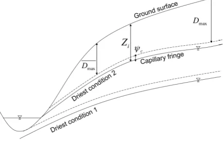
Fig. 1. Schematic hillslope section. Dmaxis the average storage deficit under the driest condition,Dmaxis the largest storage deficit under the driest condition,Zi is the water table depth, and9cthe

height of the capillary fringe.

slopes and shallow soils overlaying impermeable bedrock where topography plays a major role for runoff generation. The TOPMODEL assumptions are not valid in places with dry climate, flat terrain, or deep groundwater. The VIC model is built on fewer assumptions and is therefore easier to generalise (Kavetski et al., 2003).

The objective of this study was to provide a physically-based runoff-generation algorithm that could be used in dif-ferent global hydrological and land-surface models. The physical basis should be derived from high-resolution, glob-ally covering topographic data. The hypothesis was that the combination method of Sivapalan et al. (1997) could be ex-tended to large scales. In order to function at the global scale, the runoff-generation algorithm had to be computationally efficient and only have as many parameters as could be sub-stantiated by available data.

2 The TRG (topography-derived runoff generation) algorithm

2.1 Concepts

When water flows down a hillslope (Fig. 1), TOPMODEL assumes that the response from the groundwater system (i.e. change in water table and discharge rate) to a change in recharge/infiltration rate reaches a steady state within each time step. The temporal dynamics can then be represented by a succession of steady states. The kinematic-wave as-sumption states that the effective hydraulic gradient equals the local surface slope at every point. The two assumptions mean that the groundwater table moves up and down in par-allel. This is also an (implicit) assumption behind the VIC model.

except under surface saturation. This feature offers a way to distribute the average storage deficit to every point in the basin. In other words, the topography distribution determines the water-table distribution and thus the storage deficit. The spatial distribution of the storage deficit determines the parti-tion between fast runoff, slow runoff/baseflow, and evapora-tion when the basin wets up or dries out. The TOPMODEL steady-state assumption leads to a simple mathematical form that gives the average groundwater discharge as an exponen-tial decay function of the average storage deficit.

The consequence of the two assumptions is that a topo-graphic analysis is sufficient to derive groundwater-discharge patterns, i.e. runoff generation. As a consequence, the evolu-tion of saturated areas, water stores, and other water-balance components is strongly influenced by topography.

The meaning of storage capacity must be clearly defined in order to combine TOPMODEL and VIC concepts. The VIC model uses the term “infiltration capacity” whereas TOP-MODEL uses “deviation from average storage deficit”. An intuitive way to understand storage capacity is to define it at any location as the amount of water that can be held in vertical soil column down to the bedrock. This requires de-tailed and seldom available data of soil depths. So methods based on this definition can only be used as conceptual rep-resentations of a storage distribution. In TOPMODEL there is neither an explicit limit for the bedrock depth nor a max-imum cut-off for the storage deficit. The water-table loca-tion at each time uniquely controls the amount of water that can infiltrate before the surface is saturated and fast runoff generated. So the effective maximum storage capacity corre-sponds to the location of the deepest water table that occurs in a dry period. Here we will use the term “storage capacity” to describe the “maximum storage deficit” in TOPMODEL. 2.2 Mathematical representation of the new

combination method

We relaxed the TOPMODEL equilibrium assumption so baseflow generation should not be tied to topography. We used the topographic analysis only as a way to derive the distribution of storage capacity. The topography-derived storage distribution was fed into the VIC model framework of soil-moisture distribution to generate runoff and control evaporation. The method was constructed to differ from the original VIC model in: (1) the storage-distribution function was derived from topographic data, and as a result, there is a spatial correspondence between a storage value and a point or an area (pixel) in the basin; (2) all grid cells in the large-scale model were assigned different storage-distribution functions given by topography so each cell could be given its own aver-age storaver-age capacity; and (3) the new algorithm needed less parameters than VIC.

The storage deficitDiat any point (Fig. 1) is defined as:

Di = (Zi −9c) ·θ (1)

whereZiis the water table depth,9cthe height of the capil-lary fringe andθthe effective porosity. With the topographic index TI defined as:

TI = ln α

tanβ (2)

whereαis the upstream contributing area, andβ the local surface slope. We assumed transmissivity constant over the whole basin. The spatial distribution ofDi can then be de-rived from the average valueDby the following relationship:

Di = D +m TI −TI (3)

where TI is the area-weighted average of TI, andmis a scal-ing parameter controllscal-ing the rate of decline of transmissivity with increasing storage deficit.

Di obtained by Eq. (3) describes the profile of storage deficit under the driest condition when D takes the maxi-mum valueDmax. This defines the storage capacity in every point in the basin. The storage deficit (Di) is determined by one single moisture value (D), the topographic index, and the deepest water table in each point where the river channel acts as a boundary condition. If a basin continuously generates runoff, part of it is always saturated, i.e. has zero storage ca-pacity even under the driest condition (“Driest condition 2” in Fig. 1). When the basin is modelled as grid cells, some upstream cells may have seasonal channel or no channel at all, in which case all parts of the cell may have positive stor-age capacity. There will be a certain area in the basin that is saturated to the surface under the driest condition. If this area corresponds to a critical topographic-index value TIc, areas with values larger than this will always be saturated. In VIC, the simplification is made that the river channels are just barely saturated under the driest condition, so TIc= max(TI) (“Driest condition 1” in Fig. 1).

We defineDmax

∗

for the average storage deficit in the un-saturated area under the driest condition, i.e. with TI smaller than TIcin order to avoid the potential problem introduced by surface saturation in TOPMODEL. After insertingDmax

∗

into Eq. (3) and rearranging, we get:

Dmax

∗

= m TIc −TI (4)

wherem is a scale parameter and TI is the area-weighted average topographic index of the basin, i.e. the topographic constant.

The largest storage deficit under the driest condition, or the maximum storage capacity, is obtained by substitution of

DTI

∗

and the minimum topographic index TImininto Eq. (3):

Dmax = Dmax

∗

+m TI− TImin

= m (TIc −TImin). (5)

The storage deficit in the driest condition at every point of the water table is:

Dimax =Dmax

∗

This allowed us to define a dimensionless deficit, similar to Sivapalan et al. (1997), which is only a function of topogra-phy:

Dimax

Dmax

= TIc −TI TIc −TImin

. (7)

The actual storage capacity is scaled by parameterm. In the new algorithm it is used to scale the topographic-index range to the maximum storage capacity of the basin. Equation (7) guarantees that a given TI value will mean the same storage capacity in different grid cells in a large-scale hydrological model, and that any upstream cell without a channel will be properly represented.

2.3 Estimation of critical TI values and derivation of effective storage capacity

The operational definitions of TIc and TIminthat determine the permanently saturated area becomes crucial in the algo-rithm since they control the storage distribution. Quinn et al. (1995) present a way to define a river channel from to-pographic information and show a systematic change in TI distribution when removing the largest values representing river channels. They use a trial-and-error approach, grad-ually decreasing the channel-initiation threshold (CIT) area and allowing the channel to extend into the hillslope. The peak of the TI distribution shows a rapid shift to the left at some point, indicating upstream channels rapidly extending into the hillslope. This shifting point is reported by Quinn et al. (1995) to be the CIT value giving the best TI representa-tion.

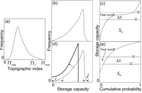
We used Eq. (6) to transfer TI values into 100 storage-capacity classes. The conversion from TI values to effec-tive storage capacity is illustrated in Fig. 2. The TI bution is first transformed into a storage frequency distri-bution, and then to a cumulative distribution. Parameteri, thei-th of the 100 storage-capacity classes represent the ef-fective extent of the river channels or permanently saturated area (Fig. 2d). We then removed saturated areas by setting all storage-capacity classes belowito zero. The driest part of the basin is represented by parameter j, thej-th of the 100 storage-capacity classes (Fig. 2d). This parameter repre-sents the maximum frequency value, used by us as a cut-off value to allow removal of the right tail of the distribution. Whenjincreases, less information from the right tail is used and the distribution gradually approaches the VIC algorithm. We tested the influence ofiandj on model performance by varying their values in ranges judged physically reasonable. The complete distribution was used wheni= 1 andj= 1 and less tail information wheniandjincreased. The range of the distribution of effective storage capacity was derived from the range of the topographic index scaled by parameterm, whereas the shape of the distribution was obtained from the distribution of the topographic index itself. The cell-average

Fig. 2. Schematic illustration of the conversion from

topographic-index distribution to storage-capacity distribution. TI_min, TIc, and

TImaxin (a) give minimum, critical, and maximum values of the

topographic index. Graphs (b) and (c) give storage-capacity distri-butions when the original information of the entire TI distribution is used, whereas (d) and (e) give the distributions when information in the 2 tails of the distributions are nullified. Parametersiandj

define the cutoff values for the two tails. In (c) and (e) the horizon-tal lines depict groundwater levels during baseflow conditions (S0 being the total storage), and during conditions of excess infiltration (1Sbeing additional storage going to fast runoff).

storage capacity was obtained by integrating the storage fre-quency distributions of all individual pixels.

2.4 Representation of water table and basin water storage

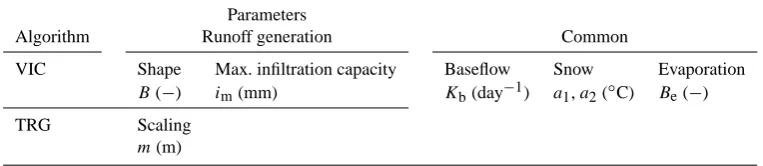
Table 1. Model parameters for the common model framework used to evaluate the VIC and TRG runoff-generation algorithms.

Parameters

Algorithm Runoff generation Common

VIC Shape Max. infiltration capacity Baseflow Snow Evaporation

B(−) im(mm) Kb(day−1) a1,a2(◦C) Be(−)

TRG Scaling

m(m)

3 Algorithm evaluation

3.1 Hydrological model framework

To compare the TRG algorithm and the corresponding VIC algorithm (Eqs. 8–9), both were inserted into the same hy-drological model framework. The framework was of a mix-ture of the one-layer version of VIC (Wood et al., 1992), to allow for distribution of the runoff generation and water storage, and WASMOD-M/WASMOD components (Wid´en-Nilsson et al., 2007; Xu, 2002), including the recently devel-oped NFR routing algorithm (Gong et al., 2009, 2010).

The VIC runoff-generation algorithm is given by:

i0 = im − im · exp



−

log− im

−im+w0+B·w0

1+ B



 (8)

A = 1 −

1− i0

im

B

(9) wherei0is the infiltration capacity,imis the maximum stor-age capacity for the saturated fraction of a model grid cell,

w0the current average storage of the cell,Athe fraction of a cell for which the storage capacity is less thani0, andB is a shape parameter. The two equations represent the partition-ing of fast and slow runoff. As a result, excess rain fallpartition-ing on saturated area will generate fast runoff.

The snow algorithm was taken from the WASMOD catch-ment model (Xu et al., 1996; Xu, 2002), whereas the evapo-ration part was given by VIC (Wood et al., 1992). The total number of model parameters was 6 for the model version using the VIC algorithm and 5 for the version using TRG (Table 1).

The NRF algorithm of Gong et al. (2009, 2010) was used to route the simulated runoff. This algorithm extracts a time-delay distribution from HydroSHEDS (Lehner et al., 2008) flow-direction data at its native resolution (300_{, around 90 m at}

the equator). The time-delay distribution is then aggregated to network-response functions for the 0.5◦ _{grid cells of the}

two hydrological models. Discharge is finally achieved by convoluting the runoff at each cell with the corresponding network-response functions.

Modelled basins were registered in the HydroSHEDS flow network overlaid with 0.5◦grid cells. Only the active part of boundary cells, as delineated by HydroSHEDS pixels, con-tributed discharge to the downstream gauging station; the rest of the boundary cells (blank area in Fig. 3) were not included. 3.2 Test basins

The performance of the two models was evaluated in 3 basins with different climates in China and North America (Figs. 3– 4). The well-documented Dongjiang (East River) basin is a tributary of the Pearl River in southern China. Its 25 325 km2 drainage area above the Boluo gauging station is large enough to retain generality of the result in a study of global hydrology. The basin has a dense network of me-teorological and hydrological gauging stations. The climate is sub-tropical with an average annual temperature of around 21◦_{C and the winter temperature only occasionally goes}

be-low zero in the mountains. The 1960–1988 average annual precipitation is 1747 mm, and the average annual runoff is 935 mm or 54 % of the average annual precipitation. About 80 % of the annual rainfall and runoff occur during the wet season from April to September. The basin is forest-covered at higher altitudes whereas intensive cultivation dominates hills and plains. Daily hydro-meteorological data, includ-ing discharge, were obtained from local sources for the Dongjiang River basin. Local daily hydro-meteorological data were retrieved for the period of 1982–1983. The Na-tional Climate Centre of the China Meteorological Adminis-tration provided data on air temperature, sunshine duration, relative humidity, and wind speed from 7 weather stations in-side or close to the basin. Precipitation data from 51 gauges and discharge data from 15 gauging stations were retrieved from the Hydrological Yearbooks of China issued by the Ministry of Water Resources. Potential evaporation was cal-culated from air temperature, sunshine duration, relative hu-midity, and wind speed with the Penman-Monteith equation in the form recommended by FAO (Allen et al., 1998).

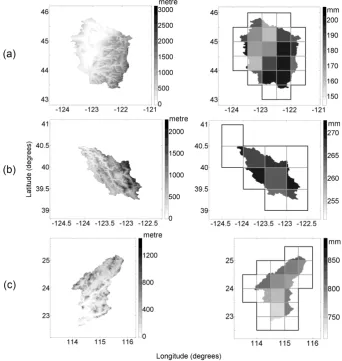
Fig. 3. Digital elevation models for (a) Willamette River basin, (b) Eel River basin, and (c) Dongjiang River basin (left row). Average storage

capacity for 0.5◦×0.5◦grid cells derived from topographic analysis for the same basins (right row). Only the active parts of the boundary cells, as delineated by HydroSHEDS pixels, were used in model calculation.

or more large flows, lasting for several days during the pas-sage of winter storms (Brown and Ritter, 1971). The Eel River at the Scotia gauging station has an area of 8062 km2. The Willamette River valley, the upstream of the Columbia River at Portland has an area of around 29 000 km2. The Willamette is mostly a gravel-bed river basin (Hughes and Gammon, 1987), which drains a humid alluvial valley with extensive active and relict floodplains (Parsons et al., 1970). The Willamette Valley lies roughly 80 km from the Pa-cific Ocean, and prevailing westerly marine winds are a pri-mary determinant of its Mediterranean climate (Taylor et al., 1994). Winters are cool and wet, summers are warm and dry. Most runoff and flooding are caused by winter rains, with winter rainfall on melting snow the primary mecha-nism for generation of floods (Waananen et al., 1971; Hub-bard et al., 1993). Melting snow at higher elevations of the Cascade Range adds a seasonal runoff component dur-ing April and May. Meteorological data from several global

remotely-sensed or reanalysis datasets were used to drive the models for the Eel and Willamette River basins. Precipita-tion data was constructed by combining TRMM (Tropical Rainfall Measuring Mission) 3B42 (Huffman et al., 2007), which has semi-global coverage from 50◦_{N to 50}◦_{S, and}

GPCP 1DD (Huffman et al., 2001) which covers the globe with 1◦resolution. TRMM provides precipitation estimation from space and involves a combination of infrared measure-ments from geostationary satellites and passive microwave measurements from polar-orbiting satellites. It has time and space scales of 3 h and 0.25◦lati◦. Air and dew-point tem-peratures were obtained from ERA-Interim reanalysis data (Simmons et al., 2007). Discharge data for Willamette and Eel River basins were taken from GRDC (2010).

3.3 Calibration of model parameters

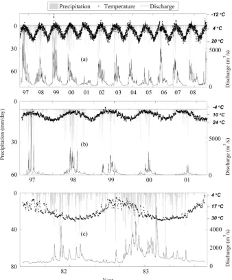
Fig. 4. Observed daily average temperature (◦C), precipitation (mm), and discharge (m3s−1) for (a) Willamette River basin, (b) Eel River basin, and (c) Dongjiang River basin. The y-axes ticks for daily average temperature show minimum, mean, and maximum values.

parameters. For each test basin, one thousand runoff time series were generated from a one thousand uniformly-distributed and randomly-combined parameter-value sets for both models. The initial snow parameter-value ranges were selected from previous modelling experiences (Wid´en-Nilsson et al., 2009). Other parameters were tuned inside their initial physical ranges before the final simulations. The 4 common parameters (Table 1) were set to the same param-eter range for both models. All paramparam-eters were calibrated with the Nash efficiency criterion, and the top 1 % parameter-value sets chosen as behavioural in the GLUE sense (Beven and Binley, 1992). Validation of VIC and TGR algorithm were performed by splitting discharge time series in half, us-ing the first half for calibration and second half for validation.

4 Results

Fig. 5. Nash efficiencies for the TRG algorithm in the Dongjiang River basin, (a) as function ofiandj, (b) as function ofiforj= 1, and (c)

as function ofjfori= 4.

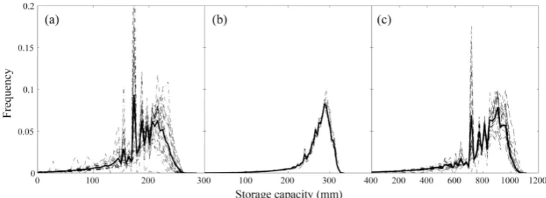
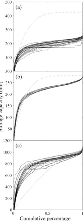
Fig. 6. Frequency distribution of effective storage capacity for whole basins (thick line) and for each individual model grid cell (dashed lines)

derived from topographic analysis for (a) Willamette River basin (b) Eel River basin, and (c) Dongjiang River basin.

4.2 Storage-capacity distributions and averages

The distributions of storage capacities, for the whole basin and for all individual grid cells, for the three river basins were all skewed to the right (Fig. 6), whereas the topographic-index distributions were always skewed to the left (Fig. 2). The skewness of the storage-capacity distributions indicated a rapid increase of storage capacity from river channel to hill-slope in all three basins. The Eel River basin showed less spatial variation in the storage distribution compared to the Willamette and Dongjiang River basins, where the distribu-tions in individual cells varied a lot from the average basin distribution. This could likely be explained by the Eel River basin being smaller and more homogeneous than the other two (Fig. 3). The spatial variability of the storage distribu-tion concerned both the cell-average storage capacity, which determines the partitioning between fast and slow runoff, and the shapes of the distributions, which define the dynamics of the partitioning. Sharp high peaks can be seen (Fig. 6) in the distributions for the Dongjiang and Willamette River basins. These peaks come from local topographic features, indicat-ing a rapid fast-runoff response in those parts of the basins.

There was a significant spatial variation in cell-average storage capacity in all three river basins, starting with a small variation along the river valleys and an increase towards headwater regions. There was also a large increase in the average basin storage capacity when going from the temper-ate North American basins to the warm and humid southern Chinese basin (Fig. 3).

4.3 Model performance

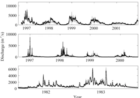
Fig. 7. Observed (gray lines) and best simulated discharge with the

TRG algorithm (black lines), and the VIC algorithm (black dots) for the Willamette River basin at Portland (top), the Eel River basin at Scotia (middle), and the Dongjiang River basin at Boluo (bottom).

0.89 for the TRG algorithm. Validation split-sample test showed similar results for the VIC and TRG algorithms. For the Dongjiang River basin, the average Nash efficiency for the validation period was 10 % higher than the calibration period for both algorithms. For Eel River basin, and the Willamette River basin, a decrease of 27 % and 15 % of Nash efficiency was observed for VIC algorithim and a decrease of 23 % and 17 % was observed for the TRG algorithm.

5 Discussion

5.1 Combined data-driven and statistical approaches O’Loughlin (1981) and Sivapalan et al. (1997) present com-bination approaches based on analytical functions fitted to the cumulative distribution of the storage capacity. By doing so, they introduce 2 or 3 parameters, which makes their so-lutions less useful for large-scale hydrological models where the lack of hydrological data is a major limitation. We limited the number of parameters by choosing a numerical instead of an analytical approach. Saulnier and Datin (2004) com-ment that the implicit neglect of surface-saturation areas in the derivation of TOPMODEL equations leads to a system-atic underestimation of catchment water storage deficit. They also show that the bias problem can potentially change the predicted ratio between surface and subsurface water fluxes. They point out that Eq. (2) is only valid for unsaturated areas. It was on the basis of this comment that we choose to develop an analytical/numerical solution to solve the bias problem. In this study, the expansion and contraction of saturated ar-eas were represented numerically, to ensure that the storage deficit was only calculated for unsaturated areas.

5.2 Where is the river?

River-channel identification is important for the implemen-tation of the TRG algorithm. The starting point for the TRG identification was taken from TOPMODEL, where the defi-nition of a river channel, or effectively the part of the basin that is always saturated, is done by assuming a cut-off CIT (channel-initiation threshold) value (Quinn et al., 1995). The parts of the basin with the largest TI values are then classified as river channels, and the TI distribution gets less positively skewed. Quinn et al. (1995) show that the optimal CIT value depends on grid resolution and that it has a significant ef-fect on the simulated basin dynamics. Quinn et al. (1995) identify the CIT value by manually finding the critical point where the number of river channels extending into the hill-slope starts to grow rapidly. They present a test of their al-gorithm on a small catchment with a 50-m DEM. We tested the same algorithm with the 90-m HydroSHEDS data. Since our pixel area was more than triple, we found that too many pixels containing river channels were included as river chan-nels started to extend into upstream areas. The trial-and-error nature of the Quinn et al. (1995) method is also unsuitable at a global scale. Our sensitivity study showed that neglecting river channels in the TRG algorithm, i.e. using i= 1 as in the VIC algorithm, gave acceptable results, but that the best results were found withi in the range 20–40 (Fig. 5). The existence or not of a river channel is a concrete real-world property and should not be considered as a free parameter but the value ofj, the cut-off CIT value for the 90-m Hy-droSHEDS data remains to be further investigated. On the basis of our 3 basins, this cut-off value was identified in a relatively narrow range. We also showed the value of main-taining the full distribution in the dry end of the spectrum, i.e.j= 1, contrary to VIC where a right tail does not exist.

The maximum storage capacity of a grid cell is propor-tional to the TI range in the unsaturated area so both max-imum and average storage capacities are reduced when the river-channel area expands. This means that a smaller part of the left tail of the storage distribution will be used to simulate basin dynamics. In the VIC model, all parts of a basin are al-located a storage capacity, and the existence of river channels is ignored. If the VIC assumptions are used (as by Sivapalan et al., 1997), that the wettest part of the basin is just barely saturated under the driest conditions then TIc= TImax. 5.3 The non-linear basin response

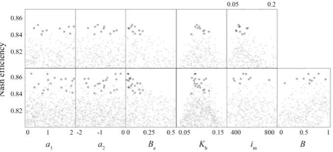
Fig. 8. Nash efficiencies as function of model parameter (gray dots) and 1 % best simulations (black circles) for the Willlamette River basin:

snow parametersa1(−) anda2(−), evaporation parameterBe(−), baseflow parameterKb(day−1), TRG scaling parameterm(m), VIC

maximum storage capacity im (mm), and VIC shape parameterB (−). The top line gives the efficiencies for the model with the TRG algorithm and the bottom line the efficiencies for the VIC-algorithm model.

The slope of the cumulative storage distribution is a key to the response of a basin to excess rainfall. A small slope means that a small rise of the groundwater table will saturate a large part of the basin thus triggering a large amount of fast runoff. The VIC storage distribution increases monotonically as a function of storage capacity whereas the TRG distribu-tion has a sharply decreasing right tail. The VIC distribudistribu-tion implies that the larger the storage capacity, the larger area it occupies in a basin. The VIC distribution results in a cu-mulative distribution with a monotonically decreasing slope (when the abscissa is probability and the ordinate is storage capacity). So basin response speeds up when the water ta-ble rises, i.e. more area gets saturated and more fast runoff is generated for a given rainfall input. The TRG distribution, derived from topographic data, always has a decreasing right tail indicating that the driest, most remote headwater areas always occupy a small part of the basin. The slope of the TRG cumulative function decreases first and then increase when the whole basin is nearly saturated (Fig. 9).

Themparameter values that gave the highest Nash effi-ciency for the TRG algorithm was used to construct a cu-mulative storage distribution for each grid cell in all three test basins. The same held true for the B andim parame-ter values for the VIC algorithm, but here for the cumulative distribution for the whole basin. The two models (VIC and TRG) happened to get the same maximum storage capacity for the Eel and Dongjiang River basins when the parame-ter values were set. The maximum storage capacities dif-fered considerably between VIC and TRG for the Willamette River basin. The cumulative TRG distribution always rose faster than VIC‘s, indicating a stronger non-linearity for runoff generation in the Eel and Dongjiang River basins. The Dongjiang River basin can be taken as example of the TRG-distribution properties. When the basin gradually wets up, a small amount of fast response will be observed initially.

A fast response will then occur when around 800 mm of the storage has been filled. Close to basin saturation, at around 1000 mm, the response speed will slow down again. The VIC distribution generates a much more linear response (Fig. 9). 5.4 Spatial variability and equifinality

The evaporation process is non-linear because of uneven dis-tribution of storage capacity, i.e. moisture available for evap-oration. A distribution that captures the real-world distri-bution should also in this case be theoretically better than one that only describes a statistical moisture distribution of a whole basin.

Stamm et al. (1994) report, in a sensitivity study of GCM-simulated global climate to representation of land-surface hydrology, that the storage capacity of the 1-layer VIC model is relatively insensitive to simulated climate in northern Eura-sia and northern America. They attribute the finding to the fact that the VIC soil moisture is not used for evaporation, but for drainage to baseflow during dry periods. This is a general problem with most single-layer land-surface models, commonly addressed by the addition of a root zone that is only depleted by evaporation and an unsaturated zone which delays the infiltration of rain water to saturated zone, or like Liang et al. (1994), the addition of the deep groundwater layer. Such structural additions add a number of parameters to a model and make it more prone to equifinality.

Fig. 9. Cumulative distributions of storage capacity for the VIC and

TRG algorithms for (a) Willamette River basin (b) Eel River basin, and (c) Dongjiang River basin.

is caused by the shape of the curve compensating the total storage amount. Other reasons could be that weather and discharge data are uncertain and that the algorithm is insen-sitive in parts of the world (Stamm et al., 1994). The TRG algorithm showed a well-determined range of behavioural values for its scaling parameterm(Fig. 8) indicating well-defined ranges for the storage distributions in the individual grid cells. The TRG algorithm thus better reflected the ac-tual spatial variation of storage capacity, both within the three river basins and between them when compared with the VIC algorithm where the storage depended on a predefined statis-tical distribution with less well calibrated parameters.

The TRG algorithm requires one parameter less than the VIC algorithm, which reduces the equifinality problem for simulated storage capacity. The cost of reducing an already low-dimensional parameter space, i.e. reducing the degrees of freedom, are diminished possibilities to adjust a model to observed discharge if the prescribed storage distribution is

wrong. This was not the case for the three basins. We could also see that the TRG algorithm was sensitive to changes in either tail of the distribution which could be taken as sign that the algorithm correctly describes the physics behind the runoff response. The large spatial variability between grid cells in a basin and between basins, as well as the reproduc-tion of local areas that affect fast and slow response differ-ently, produced by the TRG algorithm, but not by VIC, thus likely reflect real-world features (Figs. 3 and 6).

5.5 Model performance

The model using the TRG algorithm performed equally well or slightly better than the model using the VIC algorithm. It did so with one parameter less, without equifinality prob-lems, and was in the same time able to reproduce realistic spatial patterns of water storage and water available for evap-oration. Further studies are required to see if these are gen-eral features for basins worldwide and if they help in achiev-ing better performance in other models.

One crucial question concerns the applicability of the TRG algorithm in basins not fulfilling TOPMODEL assumptions, i.e. basins in dry areas, with flat terrain, and with deep groundwater. It is obvious that the cost of the diminished equifinality is lacking possibilities to tune a model where to-pographic control is weak and where it will have less con-trol on generation of fast and slow runoff, and evaporation. We relaxed the TOPMODEL assumptions and did not con-nect baseflow generation to topography. In the present model framework we already had theKb parameter to tune base-flow. In a model framework like this it should be possible to calibrate the TRG algorithm also for “non-TOPMODEL” basins.

5.6 Sensitivity of predicted discharge to the shape of storage distribution curves

Fig. 10. (a) Basin average cumulative distributions of storage capacity for Dongjiang river basin withi= 35 andi= 50. (b) Basin average relationship between the maximum storage depth and fast runoff in the Dongjiang river basin derived from (a). (c) Flow duration curve of observed discharge and TRG simulated discharge.

Fig. 11. (a) Basin average storage distribution for Dongjiang

river basin by the TRG method, and the fitted VIC model curve.

(b) Basin average relationship between the maximum storage depth

and fast runoff in the Dongjiang river basin.

The TRG-derived storage capacity distribution curve showed similarity with the VIC infiltration capacity curve, especially in the left tail before the frequency peak of the storage capacity is reached. Considering the fact that even in the humid Dongjiang basin, in more than 50 % of time less than half of the storage capacity is filled, the left tail of the storage distribution curve has more control over the predicted discharge, especially for small and medium flows. We fitted the VIC infiltration curve to left tail of the basin-average TRG storage distribution for the Dongjiang basin (Fig. 11), allowing the VIC parameter to vary until best model performance is reached and the fitting still holds. The TRG distribution showed much flatter slope as it approaches the maximum storage capacity (Fig. 11a), indicating a much flusher response to large precipitation event in the rainy sea-son (Fig. 11b). Calibrated discharge for the Dongjiang basin using both TRG storage distribution and fitting VIC infiltra-tion curve was shown in Fig. 12. The similarity in the left tail distribution of the TRG storage distribution and VIC infiltra-tion curve is clear reflected by the similarly of the simulated

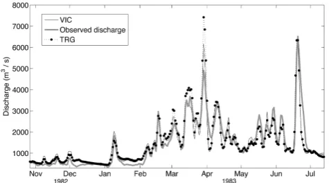
Fig. 12. Observed and simulated discharge for Dongjiang river

basin both TRG storage distribution and fitting VIC infiltration curve shown in Fig. 11.

small to medium flows; while the difference in the right tail of the two curved is shown by the distinctly higher flood peaks predicted by the TRG curve, especially in the begin-ning of the rainy reason.

6 Conclusions

the generation of fast and slow runoff, as well as evapora-tion. These facts indicate the potential for application of the TRG algorithm to model discharge in ungauged basins. More studies are needed before these results can be shown gener-ally applicable, especigener-ally in basins not fulfilling traditional TOPMODEL assumptions and when it comes to algorithms for identification of river channels.

Acknowledgements. This work was funded by the Swedish

Research Council for Environment, Agricultural Sciences and Spatial Planning, grant SWE-2005-296 from the Swedish Interna tional Development Cooperation Agency Department for Research Cooperation, SAREC, and by the Environment and Development Programme (FRIMUF) of the Research Council of Norway, project 190159/V10 (SoCoCA). Parts of the computations were performed on UPPMAX resources under Uppsala University project p2006015. We are grateful to Yongqin David Chen of the Chinese University of Hong Kong for providing hydrological data for the Dongjiang River basin. Discharge data for the Willamette and Eel River basins were provided by the Global Runoff Data Centre, 56068 Koblenz, Germany. Keith Beven is thanked for inspiring discussions that initiated this work.

Edited by: E. Morin

References

Allen, R. G., Pereira, L. S., Raes, D., and Smith, M.: Crop evapo-transpiration – guidelines for computing crop water requirements – FAO Irrigation and Drainage Paper 56, FAO, Food and Agri-culture Organization of the United Nations, Rome, 1998. Arnell, N. W.: A simple water balance model for the simulation

of streamflow over a large geographic domain, J. Hydrol., 217, 314–335, 1999.

Beven, K. and Kirkby, M. J.: Physically based, variable contributing area model of basin hydrology, Hydrolog. Sci. Bull., 24, 43–69, 1979.

Beven, K. J. and Binley, A. M.: The future of distributed models: model calibration and uncertainty prediction, Hydrol. Process., 6, 279–298, 1992.

Brown, W. M. and Ritter, J. R.: Sediment transport and turbidity in the Eel River basin, California, US Geological Survey Water-Supply Paper 1986, p.70, 1971.

Famiglietti, J. S. and Wood, E. F.: Evapotranspiration and runoff from large land areas: Land surface hydrology for atmospheric general circulation models, Surv. Geophys., 12, 179–204, 1991. Famiglietti, J. S., Wood, E. F., Sivapalan, M., and Thongs, D. J.: A

catchment scale water balance model for FIFE, J. Geophys. Res., 97(D17), 18997–19007, 1992.

Gong, L., Widen-Nilsson, E., Halldin, S., and Xu, C.-Y.: Large-scale runoff routing with an aggregated network-response func-tion, J. Hydrol., 368, 237–250, 2009.

Gong, L., Halldin, S., and Xu, C.-Y.: Global-scale river routing – An efficient delay-time algorithm based on HydroSHEDS high-resolution hydrography, Hydrol. Process., 25(7), 1114-1128, doi:10.1002/hyp.7795, 2011.

GRDC: The Global Runoff Data Centre, 56002 Koblenz, Germany, 2010.

Huffman, G. J., Adler, R. F., Morrissey, M., Bolvin, D. T., Curtis, S., Joyce, R., McGavock, B., and Susskind, J.: Global Precipitation at One-Degree Daily Resolution from Multi-Satellite Observa-tions, J. Hydrometeorol., 2, 36–50, 2001.

Huffman, G. J., Adler, R. F., Bolvin, D. T., Gu, G., Nelkin, E. J., Bowman, K. P., Hong, Y., Stocker, E. F., and Wolff, D. B.: The TRMM multisatellite precipitation analysis: quasi-global, multi-year, combined-sensor precipitation estimates at fine scale, J. Hy-drometeorol., 8, 38–55, 2007.

Hubbard, L. E., Herrett, T. A., Kraus, R. L., Ruppert, G. P., and Courts, M. L: Water resources data. Oregon water year 1993, US Geological Survey Water-Data Report OR-93-1, 1993. Hughes, R. M. and Gammon, J. R.: Longitudinal changes in fish

assemblages and water quality in the Willa- mette River, Oregon, T. Am. Fish. Soc., 116, 196–209, 1987.

Kavetski, D., Kuczera, G., and Franks, S. W.: Semidistributed hydrological modeling: a “saturation path” perspective on TOPMODEL and VIC, Water Resour. Res., 39, W1246, doi:10.1029/2003WR002122, 2003.

Lehner, B., Verdin, K., and Jarvis, A.: New global hydrography de-rived from spaceborne elevation data, EOS Trans. AGU, 89(10), 93–94, 2008.

Liang, X., Lettenmaier, D. P., Wood, E. F., and Burges, S. J.: A sim-ple hydrologically based model of land surface water and energy fluxes for general circulation models, J. Geophys. Res., 99(D17), 14415–14428, 1994.

Manabe, S., Smagorinsky, J., and Strickler, R. F.: Simulated cli-matology of a general circulation model with a hydrologic cycle, Mon. Weather Rev., 93, 769–798, 1969.

Moore, R. J. and Clarke R. T.: A distribution function approach to rainfall-runoff modeling, Water Resour. Res., 17, 1367–1382, 1981.

Nijssen, B., Lettenmaier, D. P., Liang, X., Wetzel, S. W., and Wood, E. F.: Streamflow simulation for continental-scale river basins, Water Resour. Res., 33, 711–724, 1997.

Nijssen, B., O’Donnell, G. M., Lettenmaier, D. P., Lohmann, D., and Wood, E. F.: Predicting the discharge of global rivers, J. Climate, 14, 3307–3323, 2001a.

Nijssen, B., Schnur, R., and Lettenmaier, D. P.: Global retrospective estimation of soil moisture using the variable infiltration capacity land surface model, 1980–93, J. Climate, 14, 1790–1808, 2001b. O’Loughlin, E. M.: Saturation regions in catchments and their rela-tions to soil and topographic properties, J. Hydrol., 53, 229–246, 1981.

Parsons, R. B., Balster, C. A., and Ness, A. O.: Soil development and geomorphic surfaces, Willamette Valley, Oregon, Soil Sci. Soc. Am. Proc., 34, 485–491, 1970.

Quinn, P. F., Beven, K. J., and Lamb, R.: The lna/tanb. index: how to calculate it and how to use it in the TOPMODEL framework, Hydrol. Process., 9, 161–182, 1995.

Saulnier, G. M. and Datin, R.: Analytical solution to a bias in the TOPMODEL framework balance, Hydrol. Process., 18, 1195– 1218, 2004.

Simmons, A., Uppala, S., Dee, D., and Kobayashi, S.: ERA-Interim: New ECMWF reanalysis products from 1989 onwards, ECMWF Newsletter No. 110, 25–35, 2007.

Stamm, J. F., Wood, E. F., and Lettenmaier, D. P.: Sensitivity of a GCM simulation of global climate to the representation of land surface hydrology, J. Climate, 7, 1218–1239, 1994.

Taylor, G. H., Bartlett, A., Mahart, R., and Scalley, C.: Local Cli-matological Data, Corvallis, Oregon. Oregon Climate Service, Oregon State University, Corvallis, Oregon, Report Number 911, 1994.

Waananen, A. O., Harris, D. D., and Williams, R. C.: Floods of De-cember 1964 and January 1965 in the Far Western States, US Ge-ological Survey Water-Supply Paper 1866-A, 1971.

Wid´en-Nilsson, E., Halldin, S., and Xu, C.-Y.: Global water-balance modelling with WASMOD-M: Parameter estimation and regionalisation, J. Hydrol., 340, 105–118, 2007.

Wid´en-Nilsson, E., Gong, L., Halldin, S., and Xu, C.-Y.: Model performance and parameter behavior for varying time aggre-gations and evaluation criteria in the WASMOD-M global water balance model, Water Resour. Res., 45, W05418, doi:10.1029/2007WR006695, 2009.

Wood, E. F., Lettenmaier, D. P., and Zartarian, V.: A land surface hydrology parameterization with subgrid variability for general circulation models, J. Geophys. Res., 97(D3), 2717–2728, 1992. Xu, C.-Y., Seibert, J., and Halldin, S.: Regional water balance modelling in the NOPEX area: development and application of monthly water balance models, J. Hydrol., 180, 211–236, 1996. Xu, C.-Y.: WASMOD – The water and snow balance modeling