Convex Programming Based Phase Retrieval: Theory and Applications

(1)

Convex programming-based phase retrieval: Theory and

applications

Thesis by

Kishore Jaganathan

In Partial Fulfillment of the Requirements for the Degree of

Doctor of Philosophy

CALIFORNIA INSTITUTE OF TECHNOLOGY Pasadena, California

2016

(2)

(3)

(4)

(5)

ACKNOWLEDGEMENTS

Firstly, I would like to express my sincere gratitude to my advisor Prof. Babak Hassibi. I could not have imagined having a better advisor and mentor for my Ph.D. studies. His immense knowledge, guidance, kindness and support over the years have played a crucial role in making this work possible. My understanding of many topics, including convex optimization, signal processing and entropy vectors, have significantly increased because of him. His exceptional problem solving abilities, teaching qualities and deep understanding of a wide variety of subjects have inspired me a lot. Furthermore, the intellectual freedom he offered throughout the course of my graduate studies helped me pursue my passion and grow as a research scientist. Besides my advisor, I am also extremely indebted to Prof. Yonina C. Eldar. I have been privileged to have had the opportunity to collaborate with her. Her vision and ideas have played a very important role in shaping this work. Her vast knowledge, attention to detail, work ethic and energy have influenced me significantly. Additionally, I would like to thank her for providing me the opportunity to contribute to a book chapter on phase retrieval.

I would also like to thank Prof. Palghat P. Vaidyanathan, Prof. Changhuei Yang, Prof. Joel Tropp and Prof. Venkat Chandrasekaran for serving on my defense committee. I am very grateful to Prof. Vaidyanathan for his words of wisdom, both professional and personal. I am also grateful to Prof. Yang for his valuable feedback on the practical aspects of this work, and to Prof. Tropp and Prof. Chandrasekaran for their useful convex optimization related suggestions. I would also like to express my gratitude to my undergraduate advisor and mentor Prof. David Koilpillai for being a constant source of inspiration.

(6)

from red and black in a presentation. I would also like to thank Anatoly Khina for all of the advice and conversations. The lab has been a lively place due to the energy of Ehsan Abbasi, Ramya Korlakai Vinayak and Wael Halbawi. I acknowledge the technical contributions of James Saunderson, Philipp Walk and Roarke Horstmeyer. The lunch meetings with Roarke significantly improved my understanding of the practical aspects of this work. I would like to express my gratitude to Shirley Slattery for her kind and patient administrative assistance.

I would also like to use this opportunity to thank the people who made my stay at Caltech a truly memorable one. I am forever indebted to Anupama Lakshmanan and Samet Oymak for always being there for me. To Anupama, your “bhooli bhaaliness” has added a lot of color to my life. Several of my best memories at Caltech are due to you, and I thank you for that. To Samet, I formally accept the fact that you are better than me at racquetball. Your TAing and parking skills will always be an inspiration to me.

I will always cherish the time I spent with Neel Nadkarni and Pushkar Kopparla. To Neel, thank you in advance for making the students of IIT Gandhinagar read my thesis, and for letting me travel in your Neel 45 and Neel 65 yachts. To Pushkar, thank you for introducing me to quality games like hand cricket and DotA.

The Caltech Cricket Club has been an integral part of my stay at Caltech. I would like to sincerely thank Charles Steinhardt, Siddharth Jain (and his twin brother Siddhanth Jain) and David Hall for keeping the team active, motivated and organized. I would also like to thank Sumanth Dathathri, Anantha Ravi Kiran and Sisir Yalamanchili for their camaraderie.

I would like to express my appreciation to Wong Ming Fai, Asma Qureshi, Chandni Usha (and her mother) and Harish Ravishankar for their constant support. My thanks are due to Srikanth Tenneti, Tejaswi Venumadhav and Vikas Trivedi for being accommodating roommates. I am very grateful to Rakesh Misra, Chinmoy Venkatesh, Srinidhi Tirupattur, Karthikeyan Shanmugam and Ananda Theertha Suresh for their support and encouragement.

(7)

ABSTRACT

Phase retrieval is the problem of recovering a signal from its Fourier magnitude. This inverse problem arises in many areas of engineering and applied physics, and has been studied for nearly a century. Due to the absence of Fourier phase, the available information is incomplete in general. Classic identifiability results state that phase retrieval of one-dimensional signals is impossible, and that phase retrieval of higher-dimensional signals is almost surely possible under mild conditions. However, there are no efficient recovery algorithms with theoretical guarantees. Classic algorithms are based on the method of alternating projections. These algorithms do not have theoretical guarantees, and have limited recovery abilities due to the issue of convergence to local optima.

Recently, there has been a renewed interest in phase retrieval due to technological advances in measurement systems and theoretical developments in structured signal recovery. In particular, it is now possible to obtain specific kinds of additional magnitude-only information about the signal, depending on the application. The premise is that, by carefully redesigning the measurement process, one could poten-tially overcome the issues of phase retrieval. To this end, another approach could be to impose certain kinds of prior on the signal, depending on the application. On the algorithmic side, convex programming based approaches have played a key role in modern phase retrieval, inspired by their success in provably solving several quadratic constrained problems.

(8)

LIST OF ILLUSTRATIONS

Number Page

1.1 A typical X-ray Crystallography or Coherent Diffraction Imaging (CDI) setup (courtesy of [260]). . . 2 1.2 A picture depicting the Fourier transforming property of lenses. . . . 3 1.3 An example of the input and output data in speckle interferometry

(courtesy of [Hir+11] and [Ran+13]). (A) A set of 10 low resolution speckle images. (B) The high resolution image of the stars is obtained through phase retrieval. . . 6 1.4 An active setup to estimate the position of objects in space (ULA =

Uniform Linear Array). . . 6 2.1 A synthetic example demonstrating the importance of Fourier phase

in reconstructing a signal from its Fourier transform. . . 9 3.1 Probability of successful signal recovery of (3.6) (with λ = 0) for

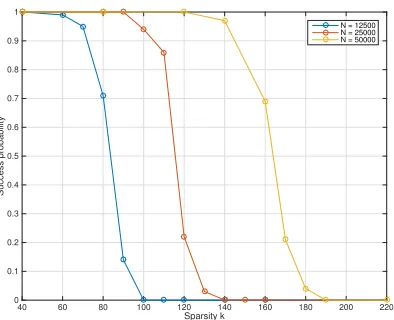
various sparsities for N = 32,64,128,256. . . 20 3.2 Probability of successful signal recovery of TSPR for various

sparsi-ties and N =12500,25000,50000. . . 31 3.3 Failure probability of TSPR for various N andθ= 0.42,0.44,0.46. . 31 3.4 Probability of successful signal recovery of various efficient sparse

phase retrieval algorithms for various sparsities and N =6400. . . 32 3.5 Probability of successful signal recovery of various SDP based sparse

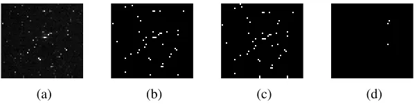
phase retrieval algorithms for various sparsities and N =64. . . 33 3.6 Reconstruction of sparse images using TSPR. (a) A 54 × 64

im-age of the M73 asterism in the constellation of Aquarius (courtesy of [NCK]). (b) A 44-sparse binary image obtained using hard-thresholding. (c) Output of TSPR. (d) Reconstruction error, after accounting for trivial ambiguities. . . 33 4.1 A typical setup for phase retrieval using masks (courtesy of [CLS15a]). 36 4.2 A pictorial example of the implementation of a simple mask in an

(11)

4.3 An example of measurements using the proposed mask designs. (a) The autocorrelation of the signalsxandx₁are obtained as

measure-ments. (b) The autocorrelation of the signalsx,x₁andx₂are obtained

as measurements. . . 44 4.4 A 2D example of measurements using Design #2. The 2D

autocor-relation of signalsx₁,x₂andx₃are obtained as measurements. . . 47

4.5 NMSE vs SNR of the SDP method for (a) Design #1 (b) Design #2. . 48 5.1 Sliding window interpretation of the STFT for N = 7, W = 5 and

L = 4. The shifted window overlaps with the signal for 3 shifts, and hence R=3 short-time sections are considered. . . 51 5.2 A typical ptychography setup (courtesy of [Nas+14]). . . 52 5.3 Fourier ptychography setup (courtesy of [ZHY13]). . . 53 5.4 Probability of successful recovery, for N = 32,M =4L, and various

choices of{L,W}, in the noiseless setting (white region: success with

probability 1, black region: success with probability 0). . . 64 5.5 Probability of successful recovery using STliFT forN = 32,W = 16,

and various choices of{L,M}(white region: success with probability

1, black region: success with probability 0). . . 65 5.6 NMSE (dB) vs SNR (dB) in the noisy setting for N =32, M = 2W. . 66 6.1 Rayleigh criterion: If two locations with nonzero values are located

such that the first zero of one sinc coincides with the maximum of the other, then the signal is barely resolvable (courtesy of [Hyp]). . . 67 6.2 A schematic representation of structured illuminations in an optical

setting. . . 69 6.3 Implementation of the proposed additional magnitude-only

measure-ments in the Direction of Arrival Estimation setup (ULA=Uniform Linear Array). . . 71 6.4 Probability of successful recovery for N = 32, R = 1, and various

choices of M and∆(x₀). . . 77 6.5 Stability of the SDP algorithm in the noisy setting for N = 32,

(12)

LIST OF TABLES

Number Page

(13)

C h a p t e r 1

MOTIVATION

Phase retrieval is the problem of recovering a signal from themagnitudeof its Fourier transform. This inverse problem has a rich history [Pat34; Pat44], motivated by applications such as X-ray crystallography [Mil90], optics [Wal63] and astronomy [FD87], where the measurable quantity is the magnitude-square of the Fourier transform of the signal of interest. In applications such as radar [GZW88] and blind channel estimation [Bay04; Ton+95], measuring the Fourier magnitude-square of the signal of interest is significantly easier than measuring the Fourier phase. In such settings, phase retrieval leads to simple and cost-effective measurement systems. In the rest of this chapter, we briefly describe the origin of phase retrieval in various applications.

1.1 X-ray Crystallography/ Coherent Diffraction Imaging

X-ray crystallography is a technique used to identify molecular and atomic structures of crystals. This method has been used to identify the structure and function of many basic molecules, including table salt [Bra13], DNA [W+53] and proteins [Dre07]. A typical experimental setup, courtesy of [260], is detailed in Fig. 1.1. A focused monochromatic X-ray beam is incident on the crystal whose structure one wishes to determine. The crystal causes the incident beam to diffract in a specific manner. By rotating the crystal, multiple two-dimensional diffraction patterns are recorded using photosensitive films or CCD cameras. A three-dimensional picture of the density of the electrons is then reconstructed from these measurements by solving an inverse problem.

(14)

[image:14.612.219.399.72.202.2]

Figure 1.1: A typical X-ray Crystallography or Coherent Diffraction Imaging (CDI) setup (courtesy of [260]).

densitiesψ(x,y,z) for all z. The quantityψtr ans(x,y)is well-approximated by the

line integral ofψ(x,y,z)along thez direction [Goo05a], i.e.,

ψtr ans(x,y) =

Z

ψ(x,y,z)dz.

The wave at(x0,y0), due to a unit point source at(x,y), is given by the scalar Green’s function

ei2λπ

√

(x−x0₎₂₊₍_y−y0₎₂₊_z0₂

4πp

(x− x0₎2+ ₍_y₋ _y0₎2+ _z02, (1.1) where λ is the wavelength [Goo05a]. Therefore, the wave at (x0,y0), denoted by

ψdi f f(x0,y0), is such that

ψdi f f(x0,y0) ∝ "

ψtr ans(x,y)

ei2λπ

√

(x−x0₎2₊₍_y−y0₎2₊_z02

p

(x−x0₎2+₍_y₋ _y0₎2+_z02dxdy.

The Fraunhofer approximation (also known as the far field approximation) involves the following steps: Thep

(x−x0₎2+₍_y₋_y0₎2+_z02term is approximated by_z0₊

x02+y02₋₍₂_{x x}0₊₂_{y y}0₎

2z0 , which holds when z

0

x−x

0 and z 0 y−y

0

(detectors sufficiently far away). The p

(x− x0₎2+ ₍_y₋ _y0₎2+ _z02 term in the denominator is further approximated by z0, which holds when

z 0

x−x

0 and z 0 y−y

0

(object restricted to a small region). Consequently, the waveψdi f f(x 0_,

y0)is Fraunhofer-approximated by

ψFr aunho f er

di f f (x

0_,

y0) ∝ e

i2_λπz0

z0 e

iπ_λx02_z+0y02

"

ψtr ans(x,y)ei

2π λ −x

0_x−y0_y z0 _dxdy.

(15)

[image:15.612.221.388.71.193.2]

f

Figure 1.2: A picture depicting the Fourier transforming property of lenses.

to the intensity of the light wave. Therefore, the diffraction pattern measurements correspond to

I(x0,y0) ∝

"

ψtr ans(x,y)ei

2π λ −x

0_x−y0_y z0 _dxdy

2

∝

$

ψ(x,y,z)ei2λπ−x

0_x−y0_y−₀_z0_z

z0 _dxdy_dz

2

∝

ˆ

ψ x0 λz0,

y0 λz0,0

! 2

, (1.2)

where ˆψis the three-dimensional Fourier transform ofψ. Hence, the measurements correspond to the magnitude-square of the three-dimensional Fourier transform of the underlying signal, along a two-dimensional plane. By rotating the crystal, the magnitude-square along various two-dimensional planes of the three-dimensional Fourier transform are obtained. The electron density is then reconstructed by solving the phase retrieval problem.

1.2 Optics

The propagation of light through a lens is an essential part in many imaging systems. The phase retrieval problem arises in such setups due to the Fourier transforming property of lenses, i.e., if a transmissive object is placed one focal length in front of a lens, then its Fourier transform is formed one focal length behind the lens [Goo05b]. A pictorial representation of this property is provided in Fig. 1.2.

(16)

the lens, denoted byψ−(x0,y0), is then given by

ψ−(x0,y0) =

"

ψ(x,y) e

i2_λπ

√

(x−x0₎₂₊₍_y−y0₎₂₊_f₂

p

(x− x0₎2+₍_y₋_y0₎2+ _f2dxdy,

using the steps described in the previous section (superposition principle, along with the scalar Green’s function (1.1)).

The Fresnel approximation (also known as the near field approximation) involves the following steps: The p

(x−x0₎2+₍_y₋ _y0₎2+ _f2 term is approximated by f + x02+y02−(2x x₂0+_f2y y0)+x2+y2, which holds when

f

x− x

0 and f y− y

0 (object restricted to a small region). The p

(x− x0₎2+ ₍_y₋ _y0₎2+ _f2 term in the denominator is further approximated by f. Consequently, the Fresnel-approximated wave is given by

ψFr esnel

− (x 0_,

y0) ∝ei

π λx

0₂₊_y0₂ f

"

ψ(x,y)ei2

π λ −x

0_x−y0_y f _ei

π λx

2₊y2 f _dxdy.

If the lens is thin, then the incoming wave at (x0,y0) leaves at (x0,y0). Due to the fact that waves travel slower in a refractive medium when compared to free space, the wave at(x0,y0)undergoes a phase delay proportional to the thickness of the lens at (x0,y0). The phase shift at (x0,y0) is calculated, using paraxial approximation [Goo05b], to be proportional toe−iπλx

02₊_y02

f . Therefore, the wave immediately after

the lens is given by

ψFr esnel

+ (x0,y0)∝

"

ψ(x,y)ei2λπ−x

0_x−y0_y f _ei

π λx

2₊y2 f _dxdy.

The Fresnel-approximated wave at the detector is hence given by

ψFr esnel di f f (x

00_,

y00) ∝ eiπλx

002₊_y002 f

"

ψFr esnel

+ (x0,y0)ei 2π

λ −x

00_x0−y00_y0 f _ei

π λx

02₊_y02

f _dx0_d_y0,

which, upon substitution and integration with respect to x0andy0, gives ψFr esnel

di f f (x

00_,

y00) ∝

"

ψ(x,y)ei2λπ−x

00_x−y00_y f _dxd_y

∝ψˆ x

00

λf,

y00 λf !

, (1.3)

(17)

1.3 Astronomy

In optical astronomy, objects in space are imaged using a ground based telescope. Even at the best observation sites, the image resolution is typically limited by atmospheric turbulence. This is due to refractive index variations of the atmosphere [FD87].

LetO(x,y)denote the object intensity one wishes to estimate. IfI(x,y)denotes the intensity measurements obtained using a telescope, then we have

I(x,y) =O(x,y)∗ p(x,y)

2_,

where p(x,y)

2_{is the point spread function introduced by the atmosphere [Har98].} In the spatial frequency domain, this relationship is equivalent to

ˆ

I(x0,y0) =Oˆ(x0,y0)Pˆ(x0,y0),

where ˆI(x0,y0), ˆO(x0,y0)and ˆP(x0,y0)are the spatial Fourier transforms ofI(x,y), O(x,y)and

p(x,y)

2_{respectively.}

It is well established that, when the measurements are taken at short exposures (in order to “freeze” the atmosphere), the atmospheric turbulence primarily affects the phase of ˆP(x0,y0), and that

ˆ

P(x0,y0) 2

obeys the same statistics across measurements with similar atmospheric conditions [Fri66]. A popular technique called speckle interferometry [Lab70] uses this fact to extract high spatial frequency information from such measurements. It involves collectingRmeasurements at short exposures under similar atmospheric conditions, so that we have

ˆ

Ir(x0,y0) =Oˆ(x0,y0)Pˆr(x0,y0) for r =1,2, . . . ,R.

Consequently, we have

* . , 1 R R X

r=1

ˆ

Ir(x0,y0) 2 + / -= ˆ

O(x0,y0) 2 * . , 1 R R X

r=1

ˆ

Pr(x0,y0) 2 + / -. (1.4)

The term 1

R

PR

r=1 ˆ

Ir(x0,y0) 2

is calculated from the measurements and the term 1

R

PR

r=1 ˆ

Pr(x0,y0) 2

is reliably estimated by observing a point object under similar atmospheric conditions1. Therefore, the quantity

ˆ

O(x0,y0) 2

is reliably obtained from these measurements. The object intensity O(x,y) is then reconstructed by solving the phase retrieval problem.

1_{The average} 1 R

PR

r=1Iˆr(x0,y0)does not provide useful information due to the fact that ˆPr(x0,y0)

(18)

[image:18.612.106.528.75.174.2]

Figure 1.3: An example of the input and output data in speckle interferometry (courtesy of [Hir+11] and [Ran+13]). (A) A set of 10 low resolution speckle images. (B) The high resolution image of the stars is obtained through phase retrieval.

1.4 Direction of Arrival (DoA) Estimation

The need for estimating the direction of wave propagation arises in many appli-cations, including radar [Zha+10], wireless communications [God97] and object tracking [RSZ94]. An active setup involves a transmitter which transmits narrow-band waves (with center frequencyωc = 2π_λc) and an array of, sayM, receivers.

Consider the two-dimensional setup such that the transmitter and receivers are placed along the x-axis at the origin and x = (λ₂, 2₂λ, . . . , M₂λ) respectively, and the transmission is uniform in the positiveyhalf of the two-dimensional space (see Fig.

1.4). Suppose there areKobjects which reflect the transmitted wave, where the kth object is located at a distancerk and an angleθk from the origin.

transmi(er* _ULA*

/2

Figure 1.4: An active setup to estimate the position of objects in space (ULA = Uniform Linear Array).

[image:18.612.204.415.449.602.2]

(19)

have

x(t)[m]=

K

X

k=1

s*

,

t− 2rk−

mλ

2 sinθk

c +

-e

iωc*

,

t−2rk−

mλ 2 sinθk

c +

-ρk,

where ρk is a function of the reflectivity of the object and its distance from the

transmitter [TF09]. Here, we use the fact that the total distance travelled by the wave reflected by the kth object onto the mth receiver is well-approximated by 2rk − m₂λsinθk. Since s(t) is slowly varying (base-band assumption), the quantity

s t− 2rk− mλ

2 sinθk

c

!

is approximated by s(t). In the frequency domain, this leads to the following relationship:

y(ω)[m]=

K

X

k=1

ˆ

s(ω−ωc)e−iωc

2rk−m_{2 sin}λ θ_k c ρ_k

∝

K

X

k=1

eiπmsinθk

ρke−

i2ω_{c rk}

c

, (1.5)

where ˆs(ω) is the Fourier transform of s(t). Therefore, the vectory corresponds

to the M low-frequency terms of the Fourier transform of a signal which has an amplitude ρke−

i2ω_{c rk}

c at location sinθk

2 , for 1 ≤ k ≤ K. The inverse problem of recovering the variousθkfromyis referred to as direction of arrival estimation (also

commonly known as super-resolution). Classic algorithms to solve this problem include MUSIC [Sch86] and ESPRIT [RK89].

This setup requires coherent detection, i.e., the receivers must be perfectly synchro-nized and be able to measure the phase of the incoming wave accurately. In practice, this is very difficult to achieve, particularly when the number of receivers is large. The measurements, due to such errors, are of the form

y[m]∝ eiφm

K

X

k=1

eiπmsinθk

ρke−

i2ω_{c rk}

c

,

for some unknownφm. A potential approach to overcome this issue is to discard the

phase measurements and only consider the magnitude measurements, i.e.,

Z[m]∝

K X

k=1

eiπmsinθk

ρke−

i2ω_{c rk}

c 2 .

(20)

C h a p t e r 2

INTRODUCTION

In this chapter, we mathematically set up the phase retrieval problem, and provide an overview of the classic and the modern approaches. For the sake of exposition, we consider the discretized 1D setting1. Letx= (x[0],x[1], . . . ,x[N−1])T be a signal of lengthN. Denote byy= (y[0],y[1], . . . ,y[N−1])T its Npoint Discrete Fourier Transform (DFT) and letZ= (Z[0],Z[1], . . . ,Z[N−1])T be the Fourier magnitude-square measurements (i.e.,Z[m]=

y[m]

2_{). Phase retrieval is the following recovery} problem:

find x (2.1)

subject to Z[m]= hfm,xi

2 _{for 0} _≤ _m _≤ _N₋₁_,

where fm is the conjugate of the mth column of the N point DFT matrix, with

elements {ei2πmnN }N−1

n=0, and h., .i is the standard inner product operator. Since

Fourier magnitude-square (i.e., power spectral density) and circular autocorre-lation are Fourier pairs, phase retrieval can also be equivalently stated as the problem of recovering a signal from its circular autocorrelation, denoted by b = (b[0],b[1], . . . ,b[N −1])T, i.e.,

find x (2.2)

subject to b[m]=

N−1 X

n=0

x[n]x?[(n+m)mod N] for 0 ≤ m ≤ N−1.

2.1 Uniqueness

Due to the absence of Fourier phase information, the available data is highly incom-plete. For any given Fourier magnitude, the Fourier phase can be chosen from an N-dimensional set. Since distinct phases correspond to different signals in general, the feasible set of (2.1) is an N-dimensional manifold, rendering phase retrieval a very ill-posed problem.

In fact, it is well known that the Fourier phase quite often contains more information than the Fourier magnitude. To demonstrate this fact, a synthetic example is provided

1_{The theory and algorithms developed in this work generalize to higher dimensions. We provide}

(21)

[image:21.612.135.478.76.221.2]

Figure 2.1: A synthetic example demonstrating the importance of Fourier phase in reconstructing a signal from its Fourier transform.

in Fig. 2.1. The figure shows the result of the following numerical simulation: Two images (of Alisha and Babu2) are Fourier transformed, their Fourier phases are swapped and then they are inverse Fourier transformed. The result clearly demonstrates the importance of Fourier phase.

A popular approach to mitigate the ill-posedness of phase retrieval is to use an M > N point DFT. In practice, this is done by increasing the density of the detectors. A typical choice is M = 2N. This setting is mathematically equivalent to zero-padding the signal xwith N zeros, and considering the 2N point DFT of (x[0],x[1], . . . ,x[N −1],0,0, . . . ,0)T. The term oversampling is used to refer to this setting.

Phase retrieval with oversampling can therefore be stated as the problem of recov-ering a signal from its autocorrelation, denoted bya= (a[0],a[1], . . . ,a[N −1])T, i.e.,

find x (2.3)

subject to a[m]=

N−1−m

X

n=0

x[n]x?[n+m] for 0 ≤ m ≤ N−1.

Remark: IfM ≥ 2N, then the inverse problem is equivalent to (2.3) irrespective of the value of M. Hence, increasing the density of the detectors does not help beyond a certain point.

(22)

Trivial Ambiguities

Observe that the operations of time-shift, conjugate-flip and global phase-change on the signal do not affect the autocorrelation, or equivalently, the oversampled DFT magnitude. Indeed, if y = (y[0],y[1], . . . ,y[M −1])T is the oversampled DFT of x, theny = (y[0],ein0_y[1], . . . ,_ein₀(M−1)_y_[_M ₋_1]₎T _{is the oversampled DFT of} _x

time-shifted byn₀units,y= (y?[0],y?[1], . . . ,y?[M−1])T is the oversampled DFT of the conjugate-flip ofx, andeiφyis the oversampled DFT ofeiφx. Each of these

operations only affect the phase of the oversampled DFT.

Hence, a signal can only be reconstructed up to a time-shift, conjugate-flip and global phase without additional information. These ambiguities are referred to as trivial ambiguities, and signals obtained by these operations are considered to be equivalent. In most applications of phase retrieval, it is good enough if a signal is reconstructed up to these ambiguities. For example, in astronomy, where the underlying signal corresponds to stars in the sky, or in X-ray crystallography, where the underlying signal corresponds to atoms or molecules in a crystal, equivalent solutions are equally informative [Mil90].

In order to calculate the number of non-equivalent solutions to (2.3), we rewrite the equations in the z-transform domain. We have

A(z) = X(z)X?(z−?), (2.4) where A(z) and X(z) are the z-transforms of a andx respectively. Since A(z) = A?(z−?), if z₀ is a zero of A(z), then z₀−?is also a zero. Hence, the zeros of A(z) appear in pairs of the form(z₀,z₀−?). The reconstruction ofxfroma, or equivalently

X(z)from A(z), is known as spectral factorization, and deals with the distribution of these pairs of zeros between X(z)and X?(z−?).

The trivial ambiguities can be understood in this framework as follows: The z transform ofx time-shifted byn₀ units is X(z)zn0. Consequently, the _z transform

of its autocorrelation is given by X(z)zn0 _× _z−n₀

X?(z−?) = X(z)X?(z−?). The z transform of the conjugate-flip of x is X?(z−?), due to which the z transform of its autocorrelation is given by X?(z−?)X(z). Indeed, this solution corresponds to “wrongly” assigning the zeros in every pair of zeros. The z transform of eiφx is

eiφX(z). Therefore, theztransform of its autocorrelation iseiφX(z)×e−iφX?(z−?) = X(z)X?(z−?).

1D setting: Since X(z) is a univariate polynomial of degree N −1, it has N −1

(23)

Consequently, A(z) has N−1 pairs of zeros (rn,rn−?). For every pair(rn,r−n?), we

can either assignrn to X(z) andrn−?to X?(z−?), or assignr−n? to X(z) andrn to

X?(z−?). Hence, the total number of non-equivalent solutions is at most 2N−1. If the zeros ofX(z)are distinct, then the number of non-equivalent solutions is exactly 2N−1_{. While this is a significant improvement when compared to the number of} non-equivalent solutions of (2.2), 2N−1 _{is still a prohibitive number, due to which} phase retrieval with oversampling in 1D remains ill-posed. Additional assumptions on the signal are required in order to be able to guarantee unique reconstruction.

≥2D setting: Here, X(z₁,z₂, . . . ,zd)is a multivariate polynomial. In [HM82], it is

shown thatalmost allpolynomials in two or more variables are irreducible. Hence, in theory, almost all signals can be uniquely reconstructed, up to trivial ambiguities, by factorizing the polynomial A(z₁,z₂, . . . ,zd). Consequently, with the exception

of a set of signals of measure zero, phase retrieval in ≥2D with oversampling is a

well-posed problem.

2.2 Classic Approaches

Earlier approaches to phase retrieval were based on the method of alternating projec-tions, pioneered by the work of Gerchberg and Saxton [GS72]. The phase retrieval problem (with oversampling, i.e., M = 2N) is reformulated as the following least-squares problem:

min

x

2N−1 X

m=0

p

Z[m]−

hfm,xi

2

(2.5) subject to x[n]=0 for N ≤ n≤ 2N −1.

Here, fm is the conjugate of the mth column of the 2N point DFT matrix, with

elementsei2πmn2N. The underlying signal has nonzero values only within the interval

[0,N−1], and has a value 0 outside this interval, i.e., in the interval [N,2N −1].

The Gerchberg-Saxton (GS) algorithm attempts to minimize this non-convex ob-jective by starting with a random initialization and iteratively imposing the time domain constraints (for example, nonzero values only within the interval [0,N−1])

and Fourier domain constraints (given Fourier magnitude measurements) using pro-jections. The details of the various steps are provided in Algorithm 1.

The intuition behind the algorithm is the following: The underlying signal is known to be inS₁∩ S2, where S₁is the set of all signals which satisfy the time domain

(24)

Algorithm 1Gerchberg-Saxton (GS) Algorithm Input: Fourier magnitude-square measurementsZ Output: Estimate ˆxof the underlying signal

Initialize: Choose a random input signalx(0),` = 0 whilehalting criterion falsedo

` ← `+1

Compute the DFT ofx(`−1): y(`) = Fx(`−1)

Impose Fourier magnitude constraints: y0(`)[m]= _|y(`)[m] y(`)_[_m_]_|

√

Z[m] Compute the inverse DFT ofy0(`): x0(`) = F−1y0(`)

Impose time domain constraints to obtainx(`) end while

return ˆx←x(`)

measurements. From any signal, it is typically straightforward to calculate the projection ontoS₁orS₂. IfS₁is the set of all signals which have nonzero values

only within the interval [0,N −1], then the projection onto this set is obtained by

forcing the values outside this interval to 0. The projection onto S₂ is the signal

obtained by calculating the Fourier transform, replacing the magnitude with the measured magnitude, and taking the inverse Fourier transform.

If the setsS₁ and S₂ are both convex, then the method of alternating projections

always converges to a signal which lies inS₁∩ S₂(assuming this set is not a null

set). In the phase retrieval setup, sinceS₂ is non-convex, this method has limited

abilities. The objective function value is shown to be non-increasing with each iteration, due to which the algorithm always converges:

2N−1 X

m=0

p

Z[m]− D

fm,x(`−1)

E 2 =2

N−1 X

m=0

D

fm,x0(`)

E − D

fm,x(`−1)

E 2 = 2N−1

X

m=0

D

fm,x0(`)

E

−Dfm,x(`−1)

E 2

= kx0(`) −x(`−1)k2_F

≥ kx0(`)−x(`)k_F2 =

2N−1 X

m=0

D

fm,x0(`)

E

−Dfm,x(`)

E 2 ≥

2N−1 X

m=0

D

fm,x0(`)

E − D

fm,x(`)

E 2 = 2N−1

X

m=0

p

Z[m]− D

fm,x(`)

E 2 ,

(25)

andx(l−1)have the same Fourier phase, Parseval’s theorem, andx0(l) is closer tox(l)

when compared tox(l−1).

The converged signal is often a local minimizer of the objective function, due to the fact that S₂ is non-convex. In order to mitigate this issue, Fienup, in his seminal

work [Fie82], extended this method by introducing additional correction terms to the time domain step (see Hybrid Input-Output (HIO) algorithm [Fie82] for details). The HIO algorithm is not guaranteed to converge, and when it does converge, it may be to a local minimum. We refer the readers to [BCL02] and [Mar07] for a theoretical and numerical investigation of such methods, and to [Fie82] for a survey of classic approaches.

2.3 Modern Approaches

The classic algorithms have limited recovery abilities, and do not have theoretical recovery guarantees. Due to these reasons, phase retrieval is still an active research problem. Recent developments in measurement technologies and advances in op-timization methods have inspired a host of new approaches to phase retrieval. The modern approaches can be broadly classified into three categories:

(i) Additional prior information: Inspired by results in the area of compressed sensing [CT05; EK12; Cha+12; Tro15], various researchers have explored the idea of sparsity as a prior information on the signal. A signal of length N is said to be k-sparse if it has k locations with nonzero values and k N. The exact locations and values of the nonzero elements are not known a priori. The approach has been to develop conditions under which only one sparse signal satisfies the autocorrelation measurements, and to develop algorithms which exploit the sparsity prior.

(ii)Additional magnitude-only measurements: Technological advances have enabled the possibility of obtaining additional information about the signal. In particular, magnitude-square measurements of the form

Z[m]=

hfm,Dxi

2 _(2.6)

(26)

(iii)Random phaseless measurements: A popular trend for analysis purposes is to replace the Fourier vectors with random vectors. The measurements considered are of the form

Z[m]=

ham,xi

2_, _(2.7)

whereamis a generic measurement vector. A natural question to ask is how many and

which measurement vectors can uniquely identify the underlying signal. Another interesting problem is to identify a set of measurement vectors for which there is an efficient and stable reconstruction algorithm. Since our work focuses on Fourier vectors which naturally come up in many applications, we do not pursue this line of work. We refer the interested readers to [BCE06; Bal+09; CSV13; LV13; NJS13; EM14; Ale+14; BR15; CLS15b; Oym+15; PLR14; SR15; Tro15] for details.

Semidefinite Programming (SDP)

On the algorithmic front, one of the recent popular approaches to treat phase re-trieval problems is to use semidefinite programming methods. SDP algorithms have been shown to yield robust solutions to various quadratic-constrained optimization problems (see [Lov79; GW95] and references therein). Since phase retrieval results in quadratic constraints, it is natural to use SDP techniques to try and solve such problems. An SDP formulation of phase retrieval (2.1) can be obtained by a proce-dure popularly known aslifting: We embed xin a higher dimensional space using

the transformationX = xx?. The Fourier magnitude measurements are then linear

in the matrixX:

Z[m]= hfm,xi

2₌_x?

fmf?mx= trace(fmf?mxx

?

) =trace(fmf?mX).

Consequently, phase retrieval reduces to finding a rank one positive semidefinite ma-trixXwhich satisfies these affine measurement constraints, leading to the following

reformulation:

minimize rank(X)

subject to Z[m]= trace(fmf?mX) for 0 ≤ m ≤ N−1

X_< 0.

(27)

[RFP10], resulting in the following convex program:

minimize trace(X) (2.8)

subject to Z[m]= trace(fmf?mX) for 0 ≤ m ≤ N−1

X_< 0.

If the underlying signal is known to be sparse, then one could add an kXk₁ cost

to the objective function [CT05]. Measurements of the form (2.6) will appear as linear constraints of the form Z[m] = trace(D?fmf?mDX). The approach has been

to develop conditions under whichx₀x?₀, where x₀ is the underlying signal, is the

unique optimizer of (2.8). We refer the readers to [She+15; JEH15a] for an overview of contemporary methods.

2.4 Organization

(28)

C h a p t e r 3

SPARSE PHASE RETRIEVAL

In many phase retrieval applications, the signal of interest is naturally sparse. For example, electron microscopy deals with sparsely distributed atoms or molecules [Mil90], while astronomical imaging tends to consider sparsely distributed stars [FD87]. If it is known a priori that the signal of interest is sparse, then one could potentially solve for the sparsest solution satisfying the Fourier magnitude measurements, and be able to uniquely and efficiently identify the underlying signal up to trivial ambiguities (the trivial ambiguities cannot be resolved with a sparsity prior). Sparse phase retrieval can be mathematically written as

minimize kxk₀ (3.1)

subject to Z[m]= hfm,xi

2 _{for 0}_≤ _m _≤ _M ₋₁_,

wherek.k₀is the`₀norm which counts the number of nonzero entries of its argument,

andMis the size of the DFT. WhenM = 2N, sparse phase retrieval is equivalent to the problem of recovering a sparse signal from its autocorrelation, i.e.,

minimize kxk₀ (3.2)

subject to a[m]=

N−1−m

X

n=0

x[n]x?[n+m] for 0 ≤ m ≤ N−1.

3.1 Contributions

In this chapter, we first show that almost all signals with aperiodic support (defined in Section 3.2) can, in theory, be uniquely recovered by solving (3.2). In other words, if the signal of interest is known to have aperiodic support, then we show that the sparse phase retrieval problem is almost surely well-posed.

(29)

Related Work

In [Ran+13], it is shown that the knowledge of the autocorrelation is sufficient to uniquely identify 1D sparse signals if the autocorrelation is “collision free”, as long as the sparsity k _, 6. A signalxis said to have a collision free autocorrelation if

for all indices{i₁,i₂,i₃,i₄}such that{x[i1],x[i2],x[i3],x[i4]}_, 0, we have|i₁−i₂| _, |i₃−i₄|. In words, a signal is said to have a collision free autocorrelation if no

two pairs of locations with nonzero values in the signal are separated by the same distance. For higher dimensions, the authors show that the requirementk , 6 is not

necessary. This result has been further refined in [OE14], where it is shown thatk2−

k+1 Fourier magnitude measurements are sufficient to recover the autocorrelation. We would like to note that the collision-free property generically holds only for O(N14−)-sparse signals, whereas our uniqueness results apply for (N −1)-sparse signals. To the best of our knowledge, TSPR is the first efficient sparse phase retrieval algorithm with strong theoretical guarantees.

3.2 Uniqueness

In this section, we present our identifiability results for the sparse phase retrieval problem (3.2).

Definition: A signal is said to have periodic or aperiodic support if the locations of

its nonzero components are uniformly spaced or not uniformly spaced respectively. For example: Consider the signalx= (x[0],x[1],x[2],x[3],x[4])of length N =5.

(i) Aperiodic support: {n|x[n]_, 0} ={0,1,3}, {1,2,4}.

(ii) Periodic support: {n|x[n],0}= {0,2,4}, {0,1,2,3,4}.

We prove the following result:

Theorem 3.2.1. Let Sk represent the set of all k-sparse signals of length n with

aperiodic support, where3 ≤ k ≤ n−1. Almost all signals inSk can be uniquely

recovered by solving (3.2).

Proof. The proof technique we use is popularly known in literature asdimension counting. SinceSkrepresents the set of allk-sparse signals with aperiodic support,

(30)

cannot be uniquely recovered by solving (3.2) is a manifold with degrees of freedom less than or equal to 2k − 1 and hence, almost all signals in Sk can be uniquely

recovered by solving (3.2). The details are provided in Appendix 8.1.

Signals with sparsity k ≤2 can always be recovered by solving (3.2) (the quadratic

system of equations can be solved trivially).

Remark: Sparse signals with periodic support can be viewed as an oversampled

version of a signal which is not sparse. The sparse phase retrieval problem (3.2) reduces to the phase retrieval problem (2.3), and hence these signals cannot be uniquely recovered from their autocorrelation without further assumptions. For a detailed discussion, we refer the readers to Section II in [LV11].

3.3 Two-stage Sparse Phase Retrieval (TSPR)

In this section, we discuss the drawbacks of the standard approaches to solve (3.2) and then develop TSPR [JOH13b].

The Fienup HIO algorithm has been extended to solve sparse phase retrieval by adapting the step involving time domain constraints to promote sparsity. This can be achieved in several ways. For example, the locations with absolute values less than a particular threshold may be set to zero. Alternatively, the k locations with the highest absolute values can be retained and the rest set to zero [MS12]. In the noiseless setting, the sparsity constraint partially alleviates the convergence issues if multiple random initializations are considered and the underlying signals are sufficiently sparse. However, in the noisy setting, convergence issues still remain. In [SBE14; SBE12], a sparse optimization based greedy search method called GESPAR (GrEedy Sparse PhAse Retrieval) is proposed. Sparse phase retrieval is reformulated as the following sparsity-constrained least-squares problem:

min

x

M−1 X

m=0

Z[m]− hfm,xi

22

(3.3) subject to kxk₀ ≤ k.

(31)

support and one in the non-support), following the so-called 2-opt method [PS82]. Given the support of the signal, phase retrieval is then treated as a non-convex optimization problem, and approximated using the damped Gauss-Newton method [Ber99]. While the algorithm enjoys empirical success, there are no theoretical guarantees.

Since the solution we desire is both sparse and low rank, a natural convex approach would be to solve:

minimize trace(X)+λkXk₁ (3.4)

subject to a[m]=trace(AmX) for 0≤ m≤ N −1

X < 0,

for some regularizerλ, where the matricesAm are given by

Amgh=

                

1 if |h−g|= m= 0 1

2 if |h−g|= m, 0

0 otherwise.

(3.5)

However, this approach does not work, as the issue of trivial ambiguities (due to time-shift and conjugate-flip) is still unresolved. IfX₀= x₀x?₀ is the desired sparse

solution, then ˜X₀ =x˜₀x˜?₀, where ˜x₀is the conjugate-flipped version ofx₀,Xi =xix?_i,

wherexi is the signal obtained by time-shiftingx0byiunits, and ˜Xi = x˜ix˜?_i, where

˜

xiis the signal obtained by time-shifting ˜x0byiunits are also feasible with the same

objective value asX0. Since (3.4) is a convex program, any convex combination of

these solutions is also feasible and has an objective value less than or equal to that of

X0, because of which the optimizer is neither sparse nor rank one. One approach to

break this symmetry would be to solve a weighted`₁minimization problem, which can potentially introduce a bias towards a particular equivalent solution. Numerical simulations suggest that this approach does not help in the sparse phase retrieval setup.

(32)

Sparsity k

20 40 60 80 100 120 140 160

Success probability

0 0.1 0.2 0.3 0.4 0.5 0.6 0.7 0.8 0.9 1

[image:32.612.209.405.80.239.2]

N=32 N=64 N=128 N=256

Figure 3.1: Probability of successful signal recovery of (3.6) (with λ = 0) for various sparsities forN =32,64,128,256.

The time-shift and time-reversal ambiguities stem from the fact that the support of the signal is not known. Therefore, let us momentarily assume that we somehow know the support of the signal (denoted from now on by V, which is the set of locations of the nonzero components ofx), (3.4) can be reformulated as

minimize trace(X)+λkXk₁ (3.6)

subject to a[m]=trace(AmX) for 0≤ m≤ N −1

X[n,m]=0 if n,m<V

X _< 0.

Fig. 3.1 plots the probability of successful recovery of (3.6) (with λ = 0) against various sparsities k for N = 32,64,128,256. For a given signal length N and sparsityk, theknonzero locations were chosen uniformly at random and the signal values in the support were chosen from an i.i.d. standard normal distribution. It can be observed that (3.6) recovers the signal with very high probability in the k ≤ N₂ regime1. This observation suggests a two-stage algorithm: one where we

first recover the support of the signal and then use it to solve (3.6).

1_{This is an empirical observation. In this work, we provide recovery guarantees only for}

(33)

Algorithm 2Two-stage Sparse Phase Retrieval (TSPR) Input: Autocorrelationaof the signal of interest Output: Sparse signalxwhich has an autocorrelationa

(i) RecoverV using Algorithm 3

(ii) Recoverxby solving (3.6) withλ =0.

It is difficult to characterize the set of signals that can be reconstructed using TSPR. In order to provide recovery guarantees, we consider a probabilistic approach. In particular, we assume that the sparse signal is drawn from the Bernoulli-Gaussian distributionBN(N, θ), defined as follows:

(i) Support is chosen from an i.i.d. Ber n

Nθ N

distribution

(ii) Signal values in the support are chosen from an i.i.d. CN(0,1) distribution.

We prove the following result:

Theorem 3.3.1. If sparse signals are drawn from theBN(N, θ)distribution, where the parameter θ satisfies0 < θ ≤ 1₂ − for some constant > 0, then the failure probability of TSPR isO(N−0.1).

Proof. This is a direct consequence of Theorem 3.3.2 and 3.3.3. For convenience of notation, we define the quantity s = Nθ. Note that s controls the distribution of the sparsity of the signals. In particular, ifk denotes the sparsity of the signal, then E[k] = s. Further, the probability that an integer belongs to the support is given by s

N.

Support Recovery

Consider the problem of recovery of the support of the signalV from the support of the autocorrelation (denoted from now on byW). We will assume that if a[i] = 0, then no two elements inxare separated by a distancei, i.e.,

a[i]=0⇒ x[j]x?[i+ j]=0∀ j.

(34)

problem can be stated as

find V subject to {|i− j| |i,j ∈V}=W, (3.7) which is the problem of recovering an integer set from its pairwise distance set (also known as theTurnpike Problem2).

For example, consider the setV = {2,5,13,31,44}. Its pairwise distance set is given

by W = {0,3,8,11,13,18,26,29,31,39,42}. The Turnpike problem (and (3.7)) is

the problem of reconstruction of the setV from the setW. We refer the interested readers to [JH13] for more details.

In [SSL90], a backtracking based algorithm is proposed to solve the turnpike prob-lem. The algorithm needs multiplicity information of the pairwise distances which is not available in the phase retrieval setup, and is known to have a worst case exponentialO(2k)-complexity. In [LW88], a polynomial factorization based algo-rithm with complexityO(kd) is proposed, whered is the largest pairwise distance. [Dak00] provides a comprehensive summary of the existing algorithms for the turn-pike problem. In the following part, we will develop aO(k4)-complexity algorithm which can provably recover mostO(N12−)-sparse integer sets.

SupposeV = {v₀,v₁, . . . ,vk−1}is a set ofk integers andW = {w0,w1, . . . ,wK−1}is its pairwise distance set4.

IfV has a pairwise distance set W, then sets c±V also have a pairwise distance set W for any integer c, because of which there are trivial ambiguities. These solutions are considered equivalent, we attempt to recover the equivalent solution U ={u₀,u₁, . . . ,uk−1}defined as follows:

U =         

V −v₀ if v₁−v₀ ≤ vk−1−vk−2

vk−1−V otherwise,

i.e., the equivalent solution setUwe attempt to recover has the following properties:

(i) u₀ =0

(ii) u₁−u₀ ≤ uk−1−uk−2.

2_{Many papers consider the problem of recovering a set of integers from the multiset of their}

pairwise distances, i.e., multiplicity of pairwise distances is known. We provide a solution without using multiplicity information.

4_{The elements of}_V _and_W _{are assumed to be in ascending order without loss of generality for}

(35)

Letui j = |uj −ui|for 0 ≤ i ≤ j ≤ k −1. With this definition,W = {ui j : 0 ≤ i ≤

j ≤ k−1}andU = {u₀j : 0 ≤ j ≤ k−1}. The reason for choosing to recover the

equivalent solutionU is the following: We have the propertyU ⊆ W. Algorithm 3, in essence, crosses out all the integers in W that do not belong toU using two instances ofIntersection Stepand one instance ofGraph Step.

Algorithm 3Support Recovery: Combinatorial Algorithm Input: Pairwise distance setW

Output: Integer setUwhich hasW as its pairwise distance set 1. u₀₁ = wK−1−wK−2

2. Intersection Step usingu01: get Z = 0∪ W ∩(W +u₀₁) 3. Graph Step using(Z,W): get{u₀p: 0 ≤ p ≤t = 3

p

log(s)}(smallestt+1 integers which have an edge withu₀,k−1)

4. Intersection Step using {u₀p : 1 ≤ p ≤ t}: get U = {u0p : 0 ≤ p ≤ t − 1} ∪

W∩

Tt

p=1(W +u0p)

!

Inferringu₀₁

The largest integer inW (i.e.,wK−1) corresponds to the termu0,k−1and the second largest integer inW (i.e., wK−2) corresponds to the termu1,k−1 (due tou1−u0 ≤ uk−1−uk−2). Hence,wK−1−wK−2= u0,k−1−u1,k−1 =u01. Observe thatu01 = v01 ifv₁−v₀ ≤ vk−1−vk−2andu01 = vk−2,k−1otherwise.

Intersection Step

The key idea of this step can be summarized as follows: suppose we know the value ofu₀pfor somep, then

{u₀j : p≤ j ≤ k−1} ⊆W ∩(W+u0p),

where the set(W +u₀p)is the set obtained by adding the integeru0pto each integer

in the setW. This can be seen as follows:u₀j ∈W by construction for 0≤ j ≤ k−1.

up j ∈W by construction forp≤ j ≤ k−1, which when added byu0p, givesu0jand

(36)

The idea can be generalized to multiple intersections. Suppose we know{u₀p : 1≤

p≤ t}, we can construct{(W +u₀p): 1 ≤ p≤ t}and see that

{u₀j :t ≤ j ≤ k−1} ⊆ W∩

∩t_p₌₁(W +u₀p)

.

The idea can also be extended to the case when we know the value ofuq,k−1for some q:

{uj,k−1: 0≤ j ≤ q} ⊆ W∩(W +uq,k−1),

which can be seen as follows:uj,k−1∈Wby construction for 0 ≤ j ≤ k−1. ujq ∈W

by construction for 0 ≤ j ≤ q, which when added byuq,k−1, givesuj,k−1and hence uj,k−1 ∈(W+uq,k−1)for 0≤ j ≤ q.

Consider the exampleV = {2,5,13,31,44},W = {0,3,8,11,13,18,26,29,31,39,42}.

We haveu₀₁ = 3, because of whichW₁ = {3,6,11,14,16,21,29,32,34,42,45}and

henceW ∩W₁ ={3,11,29,42}, which contains{u₀₁,u₀₂,u₀₃,u₀₄}= {3,11,29,42}.

Graph Step

For an integer set U whose pairwise distance set is W, consider any set Z =

{z₀,z₁, . . . ,z|Z|−1} which satisfiesU ⊆ Z ⊆ W. Construct a graph G(Z,W) with

|Z|vertices (each vertex corresponding to an integer in Z) such that there exists an edge betweenzi andzj iff the following two conditions are satisfied:

(i) ∀zg,zh∈ Z,zg− zh , zi−zj unless (i, j)= (g,h)

(ii) |zi− zj| ∈ W,

i.e., there exists an edge between two vertices iff their corresponding pairwise distance is unique and belongs toW.

The main idea of this step is as follows: suppose we draw a graphG(Z,W) where U ⊆ Z ⊆ W. If there exists an edge between a pair of integers zi,zj ∈ Z, then

zi,zj ∈ U. This holds because if zi,zj <U, then since |zi − zj| ∈ W there has to

be another pair of integers inU (and hence in Z) which have a pairwise distance

|zi − zj|. This would contradict the fact that an edge exists between zi and zj in

G(Z,W).

Consider the exampleV = {2,5,13,31,44},W = {0,3,8,11,13,18,26,29,31,39,42}.

(37)

as they have a difference of 31, which belongs toW and there are no other integer pairs in Z which have a difference of 31. Hence, the only way a pairwise distance of 31 inW can be explained is if 11,42∈U.

Theorem 3.3.2. If sparse signals are drawn from theBN(n, θ)distribution, where the parameter θ satisfies0 < θ ≤ 1₂ − for some constant > 0, then the failure probability of Algorithm 3 isO(n−0.1).

Proof. The proof of this theorem is constructive, i.e., we prove the correctness of the various steps involved in Algorithm 3 with the desired probability. The outline is as follows:

Due toU ⊆ W property, we noted that Algorithm 3 aims to cross out integers inW that do not belong toU(undesired integers). The Intersection Step and Graph Step are designed such that they never cross out integers which belong toU, and cross out undesired integers with certain probabilities.

Lemma 8.2.2 provides aO

s4 n2

bound on the probability that a particular undesired integer does not get crossed out in the first Intersection Step. If 0 < θ ≤ 1₅, then

Lemma 8.2.3 shows that the support is recovered at the end of the first Intersection Step itself with the desired probability.

The Graph Step and the second instance of the Intersection Step cross out undesired integers, if any, when 1

5 < θ. Lemma 8.2.6 shows that{v0p: 1 ≤ p ≤ t = 3

p

log(s)}

can be recovered by Graph Step with the desired probability. Finally, Lemmas 8.2.4 and 8.2.5 show that the support is recovered at the end of the second Intersection Step with the desired probability. We refer the readers to Appendix 8.2 for details.

Signal Recovery (with known support)

Once the support is recovered, the signal can be recovered by solving (3.6). We use

λ=0 as the support constraints promote sparsity by themselves.

Theorem 3.3.3. If the sparse signal x₀ is drawn from the BN(n, θ) distribution, where the parameter θ satisfies 0 < θ ≤ 1₂ − for some constant > 0, then the probability that the optimizer of (3.6), withλ= 0, is notX₀= x₀x?₀ isO(n−1).

(38)

the desired probability, which is sufficient to prove the theorem asx₀x?₀is a feasible

point of (3.6).

We use the following notation: H(U) = G(U,W) (see the description of Graph Step). In other words, H(U) is a graph with k vertices, where each vertex cor-responds to an integer inU and two vertices have an edge between them if their corresponding integers have a unique pairwise distance.

The key idea is the following: If there exists an edge between vertices corre-sponding to ui and uj in the graph H(U), then X[ui,uj] can be deduced from

the autocorrelation. This is because if there is an edge between ui and uj, then

a[|ui−uj|] = x[ui]x?[uj], which by definition is X[ui,uj]. The convex program

(3.6) can be relaxed by using only such autocorrelation constraints which fix certain entries ofX(and discarding the rest), and by replacing the positive semidefinite

con-straint with the concon-straint that every 2×2 submatrix of Xis positive semidefinite,

i.e.,

subject to X[ui,uj]= a[|ui−uj|] ifui ↔uj inH(U)

X[i, j]= 0 if i,j <U

X[i,i]X[j, j] ≥ X[i,j]

2 _∀ _i

, j & X[i,i] ≥ 0 ∀i,

whereui↔ujmeans that there exists an edge between vertices corresponding toui

andujin H(U).

Note that log6₍_s₎ _≤ _k _{holds with the desired probability. The events are first} conditioned with respect to a fixedk in this interval, a union bound over all values ofk in this interval completes the bound.

Lemma 8.3.3 shows that the minimum degree of H(U), denoted by dmin(H(U)),

satisfies dmin(H(U)) > k(1− 1_t), wheret = log2(s), with the desired probability.

Hajnal-Szemeredi theorem on disjoint cliques [HS70] states that such graphs contain

k

t vertex disjoint union of complete graphs of sizet.

Lemma 8.3.1, along with a union bound, shows that the entries of the optimizer of (3.8) match with the entries ofX₀ =x₀x?₀ on each of these k_t complete graphs with

the desired probability. Consequently, the diagonal entries of the optimizer of (3.8) match with the diagonal entries ofX₀= x₀x?₀ with the desired probability.

(39)

match with the first off-diagonal entries of X₀ = x₀x?₀. Since the optimizer’s

diagonal and first off-diagonal entries are sampled from a rank one matrix, there is exactly one positive semidefinite completion, which is the rank one completion

x₀x?₀. Since the optimizer also satisfies all the constraints of (3.6),X₀= x₀x?₀ is the

unique minimizer of (3.6) with the desired probability.

We refer the readers to Appendix 8.3 for details.

3.4 Stability

In practice, the measured autocorrelation is corrupted with additive noise, i.e., the measurements are of the form

a[m]=

N−1−m

X

n=0

x[n]x?[n+m]+z[m] for 0≤ m ≤ N −1,

wherez= (z₀,z₁, . . . ,zN−1) is the additive noise. TSPR, in its pure form (support recovery using Algorithm 3), is not robust to noise as the u₀₁ identification step and Graph Step are not robust. In this section, we present a modified version of TSPR, which in essence, considers the pairwise distance set of the pairwise distance set to identify ui₀j₀, for some 0 ≤ i0 < j0 ≤ 2c + 1, robustly and then uses a

sequence ofgeneralized Intersection Steps to provably recover the true support of mostO(n14−)-sparse signals.

The support of the noisy autocorrelation, denoted byW†= (w₀†,w†₁, . . . ,w†_K†₋₁), can

be defined as the set of integers {n | |a[n]| ≥ τ}whereτis a threshold parameter.

LetT† ={(w_i†,w†_j) : 0≤ i < j ≤ K†−1}denote the set containing the K₂† integer

pairs formed using theK†integers inW†. LetT_sub† be a subset ofT†which contains all the integer pairs(w_i†,w†_j)(where j >i), satisfying the following two conditions:

(i) w†_j −w_i† ∈W† (ii) ∃

√

K†

4 integers {g1,g2, . . . ,g√K† 4

}, such that gl,gl +w_j†−w_i† ∈T† for 1 ≤

l ≤

√

K†

4 .

The first condition requires that the difference between the integers in the pair should be in W† and the second condition requires that at least

√

K†

4 integer pairs in W† should be separated by the same difference.

(40)

Algorithm 4Two-stage Sparse Phase Retrieval: Noisy Setup

Input: Noisy autocorrelation a of the signal of interest, threshold τ, η such that kzk₂ ≤ η, constantc

Output: Sparse signal ˆxsatisfying the noisy autocorrelation measurements

(i) W† ={n | |a[n]| ≥ τ}

(ii) ui₀j₀ = wmax† −w

†

min, where 0 ≤ i0 < j0 ≤ 2c+1: w

†

min is the largest integer

for which there exists an integerw†max > w

†

minsuch that (w

†

min,w

†

max) ∈T

†

sub

(iii) Intersection Step using ui₀j₀: get {ui₀q₀,ui₀q₁, . . . ,ui₀qc+1}, where {q₀,q₁, . . . ,qc+1} ≥ (k−1)−(3c+1)(largestc+2 integers inW†∩(W†+ui₀j₀))

(iv) Intersection Step using each of the _c+2 2

terms {uqiqj : 0 ≤ i <

j ≤ c + 1}: obtain {u₀,u₁, . . . ,u√

K† 4 −1

} (largest

√

K†

4 integers in S

0≤i<j≤c+1

(W†∩(W†+uq_iq_j))+uq_jq_c₊₁

correspond to {uiq_c₊₁ : 0 ≤ i ≤

√

K†

4 −1})

(v) Intersection Step using each of the _c+2 2

terms {ui j : 0 ≤ i < j ≤ c +

1}: obtain {u√

K† 4

,u√

K† 4 +1

, . . . ,uk−1} (all the integers greater thanu√_K† 4 −1

in S

0≤i<j≤c+1

(W†∩(W†+ui j))+u0i

) (vi) ObtainX†by solving

subject to |a[m]−trace(AmX)| ≤ η for 0≤ m ≤ N−1

X[n,m]=0 if n,m _<U & X_< 0

(vii) Returnx†, wherex†x†?is the best rank one approximation ofX†

are the integers which got inserted due to a noise value higher than the threshold. Also, letWdel denote the set of integers which belong to W but do not belong to

W†: these are the integers which got deleted due to the autocorrelation value being below the threshold or due to noise reducing the autocorrelation value below the threshold. We have:

W†= (W ∪Wins)\Wdel. (3.10)

(41)

(noisy setup) can recover it from its noisy autocorrelation measurements (kzk₂ ≤ η) with an estimation error

kX†−x₀x?₀k₂ ≤ 4kη

with probability at least 1− c₀n−4, for some numerical constant c₀, if the noise vectorzand thresholdτare such that for some constantc, we have

(i) Winshas i.i.d. Ber n(p)distribution, wherep= o

s2 n

(ii) For each0 ≤ i ≤ k −1,Wdel contains at mostc terms of the form{vi j : 0 ≤

j ≤ k−1}, andv₀,k−1<Wdel.

Proof. The proof of this theorem is constructive, i.e., we prove the correctness of the various steps involved with the desired probability.

We refer the readers to Appendix 8.4 for details. The outline is as follows: Lemma 8.4.1 bounds the probability of the first step failing byO(n−4). Then, a detailed discussion of the Generalized Intersection Step is provided. Finally, Lemma 8.4.2, combined with Lemma 8.2.3, shows that TSPR (noisy setup) can precisely recover the support of the signal with the desired probability. We then show that the signal values can be robustly recovered by the convex relaxation based program.

3.5 Extension to2D

The theory and algorithms developed in this chapter can be generalized to 2Dusing the following trick: Letxbe a two-dimensional signal withN₁rows andN₂columns, andabe its two-dimensional autocorrelation with 2N₁−1 rows and 2N₂−1 columns.

Let x₁D = vec(x) denote the one-dimensional vector constructed by stacking the

columns of x on top of each other. The one-dimensional autocorrelation of x₁D,

denoted bya₁D, can be inferred froma. This can be seen as follows:

a₁D[m]=

N₁N₂−1−m

X

n=0

x₁D[n]x?₁_D[n+m]

=

N₂−1−b_Nm

1c

X