On the sources of global land surface hydrologic predictability

(1)

Hydrol. Earth Syst. Sci., 17, 2781–2796, 2013 www.hydrol-earth-syst-sci.net/17/2781/2013/ doi:10.5194/hess-17-2781-2013

EGU Journal Logos (RGB)

Advances in

Geosciences

Open Access

Natural Hazards

and Earth System

Sciences

Open Access

Annales

Geophysicae

Open Access

Nonlinear Processes

in Geophysics

Open Access

Atmospheric

Chemistry

and Physics

Open Access

Atmospheric

Chemistry

and Physics

Open Access Discussions

Atmospheric

Measurement

Techniques

Open Access

Atmospheric

Measurement

Techniques

Biogeosciences

Open Access Open Access

Biogeosciences

Discussions

Climate

of the Past

Climate

of the Past

Discussions

Earth System

Dynamics

Earth System

Dynamics

Discussions

Geoscientific

Instrumentation

Methods and

Data Systems

Open Access

_{Geoscientific}

Instrumentation

Methods and

Data Systems

Geoscientific

Model Development

Geoscientific

Model Development

Discussions

Hydrology and

Earth System

Sciences

Open Access

Hydrology and

Earth System

Sciences

Ocean Science

Discussions

Solid Earth

Discussions

The Cryosphere

Discussions

Natural Hazards

and Earth System

Sciences

Open Access

Discussions

On the sources of global land surface hydrologic predictability

S. Shukla1,*, J. Sheffield2, E. F. Wood2, and D. P. Lettenmaier1

1_{Department of Civil and Environmental Engineering, University of Washington, Seattle, WA 98195, USA} 2_{Department of Civil and Environmental Engineering, Princeton University, Princeton, NJ 08544, USA} *_{now at: Department of Geography, University of California, Santa Barbara, CA 93106, USA}

Correspondence to: D. P. Lettenmaier ([email protected])

Received: 26 January 2013 – Published in Hydrol. Earth Syst. Sci. Discuss.: 12 February 2013 Revised: 3 June 2013 – Accepted: 3 June 2013 – Published: 16 July 2013

Abstract. Global seasonal hydrologic prediction is crucial to

mitigating the impacts of droughts and floods, especially in the developing world. Hydrologic predictability at seasonal lead times (i.e., 1–6 months) comes from knowledge of ini-tial hydrologic conditions (IHCs) and seasonal climate fore-cast skill (FS). In this study we quantify the contributions of two primary components of IHCs – soil moisture and snow water content – and FS (of precipitation and temperature) to seasonal hydrologic predictability globally on a relative ba-sis throughout the year. We do so by conducting two model-based experiments using the variable infiltration capacity (VIC) macroscale hydrology model, one based on ensemble streamflow prediction (ESP) and another based on Reverse-ESP (Rev-Reverse-ESP), both for a 47 yr re-forecast period (1961– 2007). We compare cumulative runoff (CR), soil moisture (SM) and snow water equivalent (SWE) forecasts from each experiment with a VIC model-based reference data set (gen-erated using observed atmospheric forcings) and estimate the ratio of root mean square error (RMSE) of both experiments for each forecast initialization date and lead time, to deter-mine the relative contribution of IHCs and FS to the seasonal hydrologic predictability. We find that in general, the contri-butions of IHCs to seasonal hydrologic predictability is high-est in the arid and snow-dominated climate (high latitude) regions of the Northern Hemisphere during forecast periods starting on 1 January and 1 October. In mid-latitude regions, such as the Western US, the influence of IHCs is greatest during the forecast period starting on 1 April. In the arid and warm temperate dry winter regions of the Southern Hemi-sphere, the IHCs dominate during forecast periods starting on 1 April and 1 July. In equatorial humid and monsoonal climate regions, the contribution of FS is generally higher than IHCs through most of the year.

Based on our findings, we argue that despite the limited FS (mainly for precipitation) better estimates of the IHCs could lead to improvement in the current level of seasonal hydro-logic forecast skill over many regions of the globe at least during some parts of the year.

1 Introduction

Drought and floods are among the most important natural disasters globally in terms of socio-economic losses (Wilhite, 2000; Dilley et al., 2005). Since 2010, a record number of extreme drought and flood events have impacted many re-gions across the globe (Blunden et al., 2011; Blunden and Arndt, 2012) and caused enormous losses. For example, ac-cording to the US National Climate Data Center, the number of deaths and total economic losses (adjusted to 2012 USD) attributed to drought (including wild fires) and flooding, in 2010 and 2011 alone, was at least 209 and 33.6 billion USD, respectively (http://www.ncdc.noaa.gov/billions/).

Some recent studies have linked changes in the frequency and severity of natural hazards to climate change (Lau and Kim, 2012; Peterson et al., 2012; Trenberth and Fasullo, 2012) and projected a higher likelihood of occurrence of these kinds of extreme events in the future in many regions of the globe (Burke et al., 2006; Hirabayashi et al., 2008; Sheffield and Wood, 2008b; Kundzewicz et al., 2010; Dai, 2011). Global climate change and unprecedented popula-tion growth as well as industrial development has put global water resources in ever greater stress (V¨or¨osmarty et al., 2000; Oki and Kanae, 2006; Oelkers et al., 2011). There-fore, the stakes for the implementation of global hydrologic and drought prediction systems to provide outlooks for water

(2)

2782 S. Shukla et al.: On the sources of global land surface hydrologic predictability

resource conditions globally in real time are rising. Develop-ment of a Global Drought Information System was a key rec-ommendation of a World Climate Research Program work-shop “Drought Predictability and Prediction in a Changing Climate” held in 2011 (Heim and Brewer, 2012; Pozzi et al., 2013). Though thus far, the implementation of a global sea-sonal hydrologic prediction system has largely been elusive notwithstanding major strides in the last two decades in the development of large scale hydrologic models (Liang et al., 1994; Mitchell et al., 2004; Wang et al., 2009) and improve-ment in seasonal climate forecast skill (Goddard et al., 2001, 2003; Palmer et al., 2004; Saha et al., 2006; Barnston et al., 2010; Yuan et al., 2011).

Hydrologic predictability at seasonal lead times (1 to 6 months) is derived from knowledge of initial hydrologic conditions (IHCs), which includes soil moisture (SM), snow water content (SWE), ground water and surface water (Paiva et al., 2012; Singla et al., 2012; Rosenberg et al., 2013) and seasonal climate forecast skill (FS) of meteorological variables like temperature, precipitation. In the past, nu-merous studies have investigated the contributions of the IHCs and/or FS in seasonal hydrologic predictability over different regions of the globe. For example, Maurer and Lettenmaier (2003) used multiple regression to identify the sources of hydrologic predictability in the Mississippi River basin and found that initial SM was the primary source of runoff predictability at 1 month lead in all seasons except the summer months over the western mountainous region, where snow dominated the runoff predictability. In a similar study using Principal Component Analysis, Maurer et al. (2004) in-vestigated the controlling factors to the runoff predictability over all of North America and concluded that the IHCs (SM and SWE) could provide useful levels of seasonal hydrologic predictability beyond what is available via climate anomalies only. Berg and Mulroy (2006) utilized a residual analysis ap-proach and found that for a statistically significant number of stations in the Saskatchewan/Nelson River basin in Canada even macroscale estimates of initial SM could be used to im-prove streamflow predictability at 1 to 3 months lead time. Likewise Mahanama et al. (2008) showed that in the tropical island country of Sri Lanka, initial SM could contribute to the seasonal hydrologic predictability for up to 3 months lead time. They found the correlation of initial SM and monthly runoff to be the highest at 1 month lead time mainly during April-May-June (AMJ) and July-August-September with the island-wide correlation significant at 5 % significance level for 3 months lead time during AMJ. Based on their results, they concluded that improving the estimate of initial SM is far more achievable than the improvement in seasonal precip-itation forecast skill. More recently, Koster et al. (2010) and Mahanama et al. (2011) used a suite of hydrologic models to evaluate the contributions of SM and SWE to streamflow predictability across the conterminous United States. Those studies indicated that the contribution of the IHCs to seasonal

hydrologic predictability was consistent among hydrologic models.

All the studies cited above and various others not men-tioned here have addressed the question “What are the sources of seasonal hydrologic predictability and what is their relative influence?” Various methods have been used, however to our knowledge there has been no attempt to an-swer this question for the entire globe with one consistent method. Understanding the relative contributions of the IHCs and FS to seasonal hydrologic predictability at different fore-cast initialization dates and lead times globally is impor-tant for identifying those regions of the globe where use-ful skill can be attained in any given season, given current global hydrologic monitoring capability (the basis for pro-viding the IHCs) and seasonal FS. For example, depending on which one of those factors dominates the seasonal hydro-logic predictability, efforts can be focused toward improv-ing the estimation of the IHCs (e.g., by data assimilation, or model improvement that reduce prediction uncertainty in the land surface models used to estimate IHCs) or improv-ing FS. This knowledge could also lead to better understand-ing of the uncertainty of seasonal hydrologic predictability for any region and season. Hence the primary objective of this study is to provide a consistent estimate of the relative contributions of the IHCs and FS in seasonal hydrologic pre-dictability over the entire globe throughout the year. In this study we only consider the contribution of soil moisture and snow water content as IHCs. We use an ensemble stream-flow prediction (ESP) framework based on an experimental design structure proposed by Wood and Lettenmaier (2008) (described in Sect. 2.1) to conduct this analysis. ESP (Day, 1985; Wood et al., 2002; Wood and Lettenmaier, 2008; Shukla and Lettenmaier, 2011) is a method widely used for seasonal hydrologic prediction. In this method a physi-cally based hydrology model is run up to the time of fore-cast using observation-based atmospheric forcings to set ini-tial conditions. During the forecast period, the hydrology model uses ensembles of observed forcings that are resam-pled from sequences of past observations. This process re-sults in ensemble-based hydrologic forecasts that are based solely on knowledge of the IHCs (no FS). An alternative hy-pothetical structure, termed reverse ESP (Rev-ESP) by Wood and Lettenmaier (2008), runs the model up to the forecast date using ensembles of past observation-based atmospheric forcings sequences, and pairs each with observation-based atmospheric forcings (perfect FS) during the forecast period. The combination of ESP and Rev-ESP includes the two end points of no FS and perfect FS. Variations of the ESP/Rev-ESP approach have since been used in recent studies such as Li et al. (2009), Shukla and Lettenmaier (2011), Paiva et al. (2012) and Singla et al. (2012) to partition the influence of IHCs and FS on seasonal hydrologic predictability.

(3)

S. Shukla et al.: On the sources of global land surface hydrologic predictability 2783

2 Data and methods

We implemented the ESP/Rev-ESP approach to quan-tify the relative contributions of the IHCs and FS in seasonal hydrologic predictability as in previous studies (Wood and Lettenmaier, 2008; Li et al., 2009; Shukla and Lettenmaier, 2011). We conducted ESP and Rev-ESP ex-periments (Sect. 2.1) using the variable infiltration capacity (VIC) land surface model (Sect. 2.2). In each experiment we generated two distinct sets of re-forecasts (ESP and Rev-ESP based) of cumulative runoff (CR) (accumulated over 1 to 6 months lead time), soil moisture (SM) and snow wa-ter equivalent (SWE) for the entire globe during 1961–2007, for 4–6 a month long forecast periods starting on 1 January, 1 April, 1 July and 1 October. To calculate the skill of each set of re-forecasts, we used a long term consistent data set of CR, SM and SWE that was simulated by the VIC model by forcing the model with observational atmospheric forc-ings (Sect. 2.2). Then we used a simple root mean square error (RMSE) based score to quantify the skill of both exper-iments (Sect. 2.3). The ratio of the RMSE score of the two experiments was used to measure the relative contribution of the IHCs and FS to the seasonal hydrologic predictability.

2.1 Experiments

In the first experiment (ESP) the VIC model was initialized with a “true” IHC (for any given initialization day) and was forced with the ensembles of atmospheric forcings (precipi-tation, maximum (Tmax) and minimum (Tmin) temperature, wind speed) randomly sampled from the period 1961–2007 (the total number of ensembles was 46, leaving out the target year). The IHC is “true” in the context of the VIC model sim-ulation. In the second experiment (Rev-ESP) the model was initialized with ensembles of the IHCs randomly sampled from the same climatological period as in the ESP experi-ment, again leaving out the IHC of the target year. Each en-semble sequence was forced from the forecast date onwards with observed (assumed true) atmospheric forcings for the target year (equivalent to perfect climate forecast skill). The ESP experiment derives its skill from the knowledge of the IHCs only whereas the Rev-ESP experiment derives its skill solely from the observed forcings (perfect FS).

2.2 Observational analysis

We used a long-term simulated data set of CR, SM, and SWE as the reference data set to verify the skill of the ESP and Rev-ESP experiments. The availability of global, long-term and spatially distributed observations of CR, SM and SWE is scarce at best. Therefore we used the VIC model-derived simulated values of those variables, generated by forcing the model with observed atmospheric forcings, as the assumed truth for CR, SM, and SWE.

2.2.1 Atmospheric forcings

We used gridded daily precipitation, temperature maximum, temperature minimum and wind speed data developed by Sheffield et al. (2006) to drive the VIC model. Originally this data set spanned the period 1948–September 2006 (but was later extended through 2008) at one degree latitude– longitude spatial resolution and 3-hourly temporal resolu-tion. However, for the purpose of this study we spatially in-terpolated the data to 0.5◦ and temporally aggregated to a daily time step. The original Sheffield et al. (2006) data set was constructed by combining multiple ground and satellite based global observational data sets with the National Cen-ters for Environmental Prediction – National Center for At-mospheric Research (NCEP – NCAR) reanalysis. Further de-tails on the methodology involved in the generation of this data set can be found in Sheffield et al. (2006)

2.2.2 The variable infiltration capacity (VIC) model

The VIC model is a semi-distributed macroscale hydrol-ogy model that parameterizes major surface, subsurface, and land–atmosphere hydrometeorological processes (Liang et al., 1994, 1996; Cherkauer et al., 2003). The VIC model has been widely used at global scale in many previous studies and has been demonstrated to capture the hydrology of dif-ferent regimes well (Nijssen et al., 1997, 2001a,b,c; Maurer et al., 2002; Adam et al., 2007). The VIC model has also been used to successfully simulate and reconstruct hydrologic ex-tremes such as drought and floods globally (Sheffield et al., 2004; Sheffield and Wood, 2008a,b; Voisin et al., 2011; Wang et al., 2011).

The VIC model represents the role of sub-grid spatial het-erogeneity in soil moisture, elevation bands, and vegetation on runoff generation. The subsurface in the VIC model is partitioned into three layers. The first layer has a fixed depth of∼30 cm and responds quickly to changes in surface con-ditions and precipitation. Moisture transfers between the first and second, and second and third soil layers are governed by gravity drainage, with diffusion from the second to the upper layer allowed in unsaturated conditions (Liang et al., 1996). Baseflow is a nonlinear function of the moisture con-tent of the third soil layer (Todini, 1996). Each grid cell in the VIC model is divided into N+1 land cover tiles, wheren= 1 toN represents different vegetation types and N+1 land cover is bare soil. Each vegetation type has as-sociated monthly vegetation parameters such as leaf area in-dex (LAI), albedo, minimum stomatal resistance, architec-tural resistance, roughness length, relative fraction of roots in each soil layer, and displacement length. Actual evapotran-spiration in the VIC model is calculated using the Penman– Monteith equation (Shuttleworth, 1999). Total actual evapo-transpiration is the sum of canopy evaporation and transpira-tion from each vegetatranspira-tion tile and bare soil evaporatranspira-tion from the bare soil tile, weighted by the coverage fraction for each

(4)

tile. For further details about the VIC model the reader is re-ferred to Liang et al. (1994, 1996).

For this study we ran the VIC model in water balance mode. In the water balance mode the model runs at daily time step (except the snow module that was run at 3 hourly time step) and the surface energy balance is not calculated, instead assuming that the soil surface temperature is equal to the surface air temperature. The global soil, vegetation and snow band parameters used to run the VIC model were the same as used by Su et al. (2005) and Voisin et al. (2008). We conducted the model spinup by first cold starting a model run (i.e., arbitrary initial state) for the period 1948–2008 and then used the state at the end of that simulation (as of 31 De-cember 2008) to start another simulation for 1948 through 1959. Finally, we used the state at the end of that simulation (as of 31 December 1959) to initialize a simulation for 1948 through 2008 and used the model output from the simulation period 1960–2008 as the reference. Furthermore, the state files from that simulation (during the period of 31 Decem-ber 1960 through 31 DecemDecem-ber 2007) were used to initialize both experiments (ESP and Rev-ESP) for different forecast periods.

2.3 Forecast score

In order to quantify the relative contributions of the IHCs and FS on seasonal hydrologic predictability, we calculated the RMSE of both experiments and then used the RMSE ratio to partition the influence of the IHCs and FS. As in Li et al. (2009) and Shukla and Lettenmaier (2011), we estimated RMSE for each experiment by first calculating the squared error for each ensemble member, and then calculating the square root of the mean squared error. We could have used other skill scores such as anomaly correlation; however, we wanted to be consistent in our methodology with the past studies mentioned above.

We considered that when the RMSE ratio is less than 1.0 then IHCs dominate the seasonal hydrologic predictability and vice versa. Note that in what follows, we use the word “skill” to denote the “forecast skill score” of the ESP or Rev-ESP experiments as described in this section.

3 Results

In this section we present and discuss the seasonal, spatial and temporal (with lead time) variability of the relative con-tributions of the IHCs and FS in seasonal hydrologic pre-dictability across the globe. We first discuss the variation of the kappa (κ) parameter defined by Mahanama et al. (2011) and used by Shukla and Lettenmaier (2011) and then illus-trate the predictability of SM, SWE and CR, respectively, in Sects. 3.2, 3.3 and 3.4.

3.1 Variability of kappa (κ) parameter

Kappa (κ) was defined by Mahanama et al. (2011) as the ra-tio of the standard deviara-tion of total moisture (soil moisture and snow) at the time of forecast initialization to total precip-itation during the forecast period as shown below:

k=σw/σP, (1)

whereσw is the standard deviation of total initial moisture

(SM+SWE) over the hindcast period (i.e., 1961–2007 in this case) andσP is the standard deviation of the total

pre-cipitation during the forecast period (calculated at 1, 3 and 6 month leads) over the same hindcast period. We used total SM (SM summed over all three soil layers) along with SWE to estimateσw. The total depth of the three layers varied from

about 1 to 4.6 m globally.

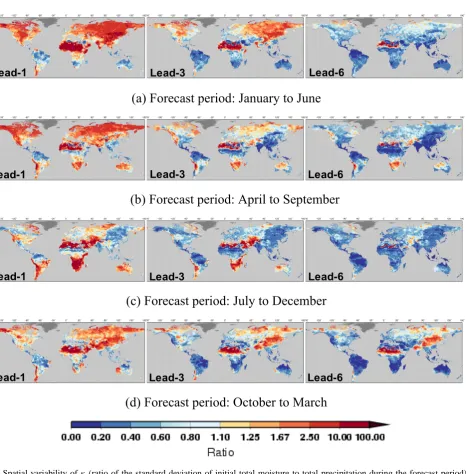
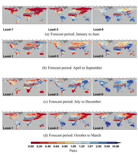
κ greater than 1 implies that variability of the initial total moisture may dominate the hydrological forecasts and the reverse is implied byκless than 1. Figure 1 shows the varia-tion ofκglobally at lead times of 1 to 6 months for forecasts starting on (a) 1 January, (b) 1 April, (c) 1 June and (d) 1 De-cember. Red colors indicate κ values greater than 1, with dark red colors indicating the highest values, whereas blue colors show the opposite (i.e., kappa values less than 1). To-tal moisture variability is higher than precipitation variability (resulting inκ greater than 1) in North America, except for the US Pacific coast, Western Mexico, and the Southeastern US. For at least 1 month lead time except in Northwestern Europe, the same is true in the rest of Europe, Russia and Asia for forecast periods starting on 1 January (Fig. 1a).κ values greater than 1 persist through lead times of 3 months over some parts of the high latitude regions of North Amer-ica (North of 50◦_{N latitude), Central US, Russia and Central} Asia. On the other hand,κvalues are below 1 in the Southern Hemisphere with the exceptions of deserts in South America for the rest of the period during the same 1 January forecast period. We can see opposite spatial patterns ofκ values in forecast periods starting on 1 July (Fig. 1c).

In the snow-dominated regions of the world (mainly in the Northern Hemisphere)κ values are higher than 1 during at least the first three months of the forecast period starting on 1 January (Fig. 1a) and on 1 April (Fig. 1b). Snowmelt con-tributes to runoff and soil moisture during the otherwise dry summer months (June to September) in those regions. Again during the forecast period starting on 1 October (Fig. 1d), κ values are greater than 1 for the regions that are dry dur-ing October to March. Regions such as northern India and Central Asia particularly stand out becauseκ >1 for up to 6 months lead time in those regions. On the contrary for re-gions such as Western US, and tropical rere-gions (∼between 23◦S to 23◦N),κ <1 starting at 1 month lead time.

In the next 3 sub-sections we describe the role of IHCs (SM and SWE only) and FS in the predictability of SM, SWE and CR, in terms of the RMSE ratio of the ESP and Rev-ESP experiments. We expected the spatial and temporal

(5)

36

794

795 (a) Forecast period: January to June

796

797 (b) Forecast period: April to September

798

799 (c) Forecast period: July to December

800

801 (d) Forecast period: October to March

802

803

804 Fig. 1: Spatial variability of κ (ratio of the standard deviation of initial total moisture to

805 total precipitation during the forecast period) at lead-1, -3 and -6 months for forecast

806 initialization on (a) 01 January (b) 01 April (c) 01 July (d) 01 October.

807

808 Lead-1

Lead-3

Lead-6

Lead-1

Lead-3

Lead-6

Lead-1

Lead-3

Lead-6

Lead-1

Lead-3

Lead-6

Fig. 1. Spatial variability ofκ(ratio of the standard deviation of initial total moisture to total precipitation during the forecast period) at lead-1, -3 and -6 months for forecast initialization on (a) 1 January, (b) 1 April, (c) 1 July and (d) 1 October.

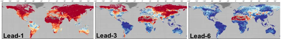
pattern of the RMSE ratio to be in general agreement withκ. Shukla and Lettenmaier (2011) also showed a first order rela-tionship betweenκ and the inverse RMSE ratio. The RMSE ratio is the ratio of RMSEESPand RMSERev-ESP; therefore,

if its value is less than 1 then it indicates that the relative contribution of the IHCs is larger than the contribution of the FS in the CR forecasts and vice versa. To quantify the co-variability between kappa and the RMSE ratio, we calcu-lated a rank based spatial pattern correlation between kappa and the inverse RMSE ratio (i.e., RMSERev-ESP/RMSEESP)

for SM and CR forecasts. This metric calculates correlations among the ranks of the data (not the actual values). Rank

based correlation metrics are more appropriate for calculat-ing correlations among inverse RMSE score and kappa be-cause they are relatively insensitive to outliers and can detect monotonic relationships that are not necessarily linear in na-ture. Results of this analysis are shown in Figs. 4 and 8. High pattern correlation between both quantities indicates that low values of kappa coincide with low values of inverse RMSE ratio globally and vice versa.

3.2 Predictability of soil moisture (SM)

Figure 2a through d show the RMSE ratio for SM forecasts at 1, 3 and 6 months lead time during the forecast period

[image:5.595.71.538.51.526.2]

(6)

37

809

810 (a)

Forecast period: January to June

811

812 (b) Forecast period: April to September

813

814

815 (c) Forecast period: July to December

816

817 (d) Forecast period: October to March

818

819

820

821 Fig. 2: RMSE ratio for soil moisture (SM) forecasts at lead-1, -3 and -6 months for

822 forecast initialization on (a) 01 January (b) 01 April (c) 01 July (d) 01 October.

823

824 Lead-1

Lead-3

Lead-6

Lead-1

Lead-3

Lead-6

Lead-1

Lead-3

Lead-6

Lead-1

Lead-3

Lead-6

Fig. 2. RMSE ratio for soil moisture (SM) forecasts at lead-1, -3 and -6 months for forecast initialization on (a) 1 January, (b) 1 April, (c) 1 July and (d) 1 October.

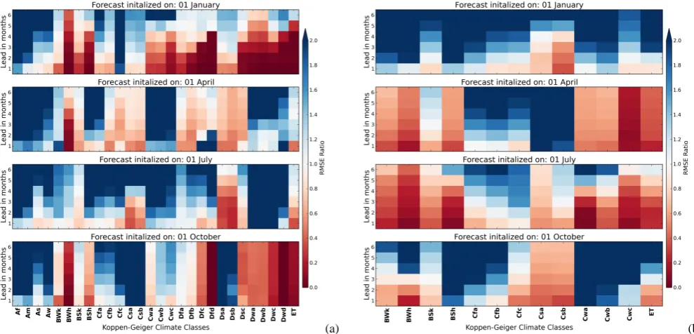
starting on 1 January, 1 April, 1 July and 1 October, respec-tively. Figure 3a and b show the median of the RMSE ra-tio for SM forecasts over different Koppen–Geiger climate classes (Kottek et al., 2006) (Table 1). Figure 3a includes all the climate classes in the Northern Hemisphere as well as equatorial climate regions and Fig. 3b shows rest of the cli-mate classes in the Southern Hemisphere.

The main pattern that stands out in these figures is the strong influence of the IHCs almost globally (with excep-tions of equatorial climate regions) at 1 month lead time, in-dicated by low values of the RMSE ratio. Shukla and Letten-maier (2011) and Mo et al. (2012) also found a predominant effect of SM persistence (hence dominance of IHCs) at short leads.

[image:6.595.57.539.64.131.2]

(7)

[image:7.595.45.541.86.427.2]

Table 1. K¨oppen–Geiger Climate Classification (source: Kottek et al., 2006).

Main climates Precipitation Temperature

A: Equatorial W: Desert h: Hot arid F: Polar frost

B: Arid S: Steppe k: Cold arid T: Polar tundra

C: Warm temperature f: Fully humid a: Hot summer D: Snow s: Summer dry b: Warm summer E: Polar w: Winter dry c: Cool summer

m: Monsoonal d: Extremely continental

38 825

(a) 826

827

(a)

39 828

(b) 829

Fig. 3: Median of RMSE ratio for SM forecasts, over the grid cells in different Koppen-830

Geiger climate classes in (a) Northern Hemisphere and Tropics and (b) Southern 831

Hemisphere (excluding Equatorial climate regions, that are included in (a)) 832

833

834

(b)

Fig. 3. Median of RMSE ratio for SM forecasts, over the grid cells in different Koppen–Geiger climate classes in (a) Northern Hemisphere and tropics and (b) Southern Hemisphere – excluding equatorial climate regions that are included in (a).

In the Northern Hemisphere the influence of the IHCs on SM predictability is particularly dominant over arid as well as snow-dominated climate regions during the forecast period starting on 1 January (Figs. 2a and 3a). In snow-dominated climate regions, the strong influence of the IHCs for up to 6 month lead times can be seen in the forecast period starting on 1 October as well (Figs. 2d and 3a). A noteworthy contrasting pattern of RMSE ratio can be seen over the equa-torial regions where the FS dominates the SM predictability almost throughout the year.

Similar to climate regions in the Northern Hemisphere, the IHCs influence SM predictability at 1 month lead time in the Southern Hemisphere as well (Figs. 2 and 3b). Overall the influence of IHCs is strongest during forecast periods start-ing on 1 April and 1 July (Figs. 2b,c and 3b), mainly over arid and temperate dry winter climate regions of the Southern Hemisphere. For the rest of the climate regions FS dominates SM predictability beyond 1 month lead time.

Figure 4 shows the rank-based pattern correlation between kappa and the inverse RMSE ratio for SM forecasts. Gener-ally the pattern correlation between both quantities is strong (>0.5), with the lowest values during the forecast period starting on 1 April. The lower correspondence between in-verse RMSE and kappa values in April may be due to the fact that by construct the inverse RMSE ratio takes into ac-count the timing of snowmelt whereas kappa does not. For example in regions with high SWE values at the beginning of the April forecast period, kappa values will tend to be high (>1) at 1 month lead simply because initial moisture vari-ability is higher than precipitation varivari-ability during the first month; however, the inverse RMSE ratio attains high values only when the snowmelt actually starts to contribute to the replenishment of the soil moisture, which may not necessar-ily happen in the first month of the forecast period depending on the elevation and temperature of the region.

(8)

40 835

Fig. 4: Pattern correlation between Kappa and inverse RMSE ratio (RMSERev-ESP/

836

RMSEESP) at lead-1, -3 and -6 months for SM forecasts initialized on 01 January, 01

837

April, 01 July and 01 October. 838

839

Fig. 4. Pattern correlation between kappa and inverse RMSE ra-tio (RMSERev-ESP/RMSEESP) at lead-1, -3 and -6 months for SM

forecasts initialized on 1 January, 1 April, 1 July and 1 October.

3.3 Predictability of snow water equivalent (SWE)

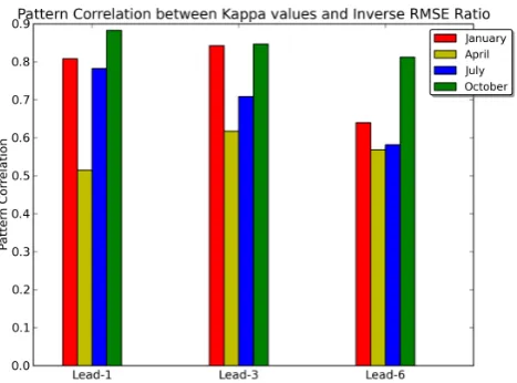
Snow plays a major role in the annual water supply for nearly half of the Northern Hemisphere (Barnett et al., 2005). In those regions snows accumulates through the winter and melts in the spring and/or summer months to replenish runoff and soil moisture. Figure 5 shows the ratio ofκ calculated using initial SM variability (κSM) and initial SWE

variabil-ity (κSWE). We focus on those grid cells only whereκvalues

(calculated using both SM and SWE variability) are greater than 1 (i.e., the regions where initial total moisture variability is higher than then total precipitation variability) and where κSWEis greater than 0.1 (grid cells where there is an

appar-ent contribution of snow to hydrologic predictability). This figure shows that during forecast periods starting in January and April the relative contribution of snow is higher than the contribution of SM (i.e., those grid cells where κSM/κSWE

is less than 1 over large parts of the high latitude regions of the Northern Hemisphere). This in turn implies that in those regions predictability of SWE is crucial to predict wa-ter supply.

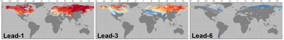
Figure 6 shows the spatial and temporal variability of the RMSE ratios for SWE forecasts during the forecast period starting on 1 January (Fig. 6a), 1 April (Fig. 6b), 1 July (Fig. 6c) and 1 October (Fig. 6d). In this figure we show those grid cells only for months for which the long-term mean SWE (calculated over 1961–2007) is higher than 50 mm. This screening based on the long-term mean values of SWE allows us to focus on those regions of the globe that re-ceive substantial amounts of snow. Figure 6 shows that at short leads the IHCs dominate the SWE forecast, which is expected because SWE is a state variable.

During the forecast period starting on 1 January, which consists of the months with highest values of SWE during most years, over the high latitude regions of Asia and North

America the IHC influence on the SWE predictability per-sists through at least 3 months lead time.

3.4 Predictability of cumulative runoff (CR)

Figure 7 shows the RMSE ratios for CR forecasts globally at 1 to 6 months lead time during the forecast period start-ing on 1 January (Fig. 7a), 1 April (Fig. 7b), 1 July (Fig. 7c) and 1 October (Fig. 7d). CR at any lead timeNis the sum of runoff during lead 1 toN months. Sinceκ at any lead time N (1, 3 and 6 months for this study as shown in Fig. 1) was also calculated using the total precipitation during lead 1 to N months (and the initial total moisture at the beginning of the forecast period). In Fig. 7 we only show the RMSE ratio for those grid cells where RMSERev-ESP or both RMSEESP

and RMSERev-ESP are greater than zero (RMSEESP and

RMSERev-ESP both could be zero for desert areas, e.g., in

Africa, Middle East, Central Asia, South America and Aus-tralia). Similar to Fig. 3, Fig. 8 shows the median values of the RMSE ratio for CR forecasts over Koppen–Geiger cli-mate classes (Table 1).

In general, in the Northern Hemisphere the influence of IHCs on CR predictability is highest during the forecast pe-riod starting on 1 January and 1 October (Figs. 7a,d and 8a). This is particularly true for arid regions (such as the inte-rior Western US and central Asia) as well as snow-dominated climate regions in the high latitudes of the Northern Hemi-sphere. In the Pacific coastal portion of the Western US, IHCs influence the CR predictability for up to 6 months lead time during the forecast period starting on 1 April (Figs. 7b and 8a) and up to 3 months during the forecast period start-ing on 1 July. Again, in the equatorial climate regions FS dominates CR predictability throughout the year.

In the arid regions and dry winter temperate climate re-gions of the Southern Hemisphere, IHCs influence the CR predictability during forecast periods starting on 1 April and 1 July (Figs. 7b,c and 8b). In the warm temperate humid re-gions of the Southern Hemisphere (in Southern America and in Eastern Australia) FS dominates CR forecast predictabil-ity almost through the year beyond 1 month lead time.

Figure 9 shows the pattern correlation between kappa val-ues and inverse RMSE ratio for CR Forecasts. In general the pattern correlation values are stronger than for SM forecasts, but the spatial variations are roughly similar.

3.5 Sensitivity analysis

The depth of the second and third soil layers in the VIC model was estimated via calibration. Given the dearth of high quality long-term observations of runoff and soil moisture, uncertainty in the calibrated soil depths is unavoidable. The soil parameters used in this study are the same as in Nijssen et al. (2001b,c). In those studies VIC parameters were eval-uated by comparing VIC simulated runoff, soil moisture and snow cover with the observations globally. The studies found

[image:8.595.51.285.60.233.2]

(9)

41

840

841 (a)

Forecast period: January to June

842

843 (b) Forecast period: April to September

844

845 (c)

Forecast period: April to September

846

847 (d)

Forecast period: October to March

848

849

850

851 Fig. 5: Ratio of κ

SM

to κ

SWE

(depicting the contribution of SM relative to SWE in seasonal

852 hydrologic predictability) at lead-1, -3 and -6 months since the forecast initialization on

853 (a) 01 January (b) 01 April (c) 01 July (d) 01 October. (The regions shaded in grey are

854 grid cells for which κ < 1 and κ

SWE

< 0.1, or the regions that do not receive snow).

855

Lead-1 Lead-3 Lead-6

Fig. 5. Ratio ofκSM toκSWE (depicting the contribution of SM relative to SWE in seasonal hydrologic predictability) at lead-1, -3 and

-6 months since the forecast initialization on (a) 1 January, (b) 1 April, (c) 1 July and (d) 1 October. (The regions shaded in grey are grid cells for whichκ <1 andκSWE<0.1, or the regions that do not receive snow.)

a reasonable agreement between the observations and VIC simulations. Nevertheless, we conducted an analysis to esti-mate the sensitivity of the results of this study to the change in the depth of the soil layer 2 and 3, since the soil depth im-pacts the water holding capacity and in turn the convergence of the Rev-ESP experiments to the control simulation.

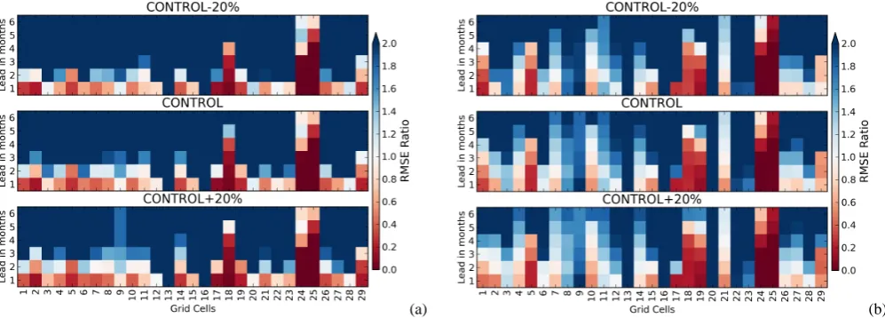
We selected 29 grid cells for this analysis (Fig. 10) that represent different climate zones across the globe. We gener-ated two sets of soil parameters by reducing the depth of soil layers 2 and 3 by 20 % [CONTROL−20 %] and by increas-ing them by 20 % [CONTROL+20 %], where CONTROL

is the nominal set of soil parameters used in all other exper-iments. We then performed ESP and REV-ESP experiments for each set of soil parameters in the same manner as de-scribed in Sect. 2.1. We also generated reference data sets using both sets of soil parameters (as mentioned in Sect. 2.2). Figures 11 and 12 compare the RMSE ratios obtained by the CONTROL−20 %, CONTROL and CONTROL+20 % experiments for SM and CR forecasts, made during forecast periods starting 1 January and 1 July. From those figures it is clear that the impact of change in soil depth on the RMSE ratio is minimal. In general, changes in the RMSE ratio occur

[image:9.595.58.534.54.516.2]

(10)

42

856

857 (a)

Forecast period: January to June

858

859 (b) Forecast period: April to September

860

861 (c)

Forecast period: July to December

862

863 (d) Forecast period: October to March

864

865

866 Fig. 6: RMSE ratio for Snow Water Equivalent (SWE) forecasts at lead-1, -3 and -6

867 months since the forecast initialization on (a) 01 January (b) 01 April (c) 01 July (d)

868 01 October. (The regions shaded in grey are grid cells for which long term mean

869 SWE is less than 50 mm).

870 Lead-1

Lead-3

Lead-6

Lead-1

Lead-3

Lead-6

Lead-1

Lead-3

Lead-6

[image:10.595.58.537.64.132.2]

Lead-1

Lead-3

Lead-6

Fig. 6. RMSE ratio for snow water equivalent (SWE) forecasts at lead-1, -3 and -6 months since the forecast initialization on (a) 1 January, (b) 1 April, (c) 1 July and (d) 1 October. (The regions shaded in grey are grid cells for which long-term mean SWE is less than 50 mm.)

mostly it in the middle range of 0.6 to 1.4 for the CONTROL experiment, meaning when neither IHCs nor FS dominates the seasonal hydrologic predictability.

4 Discussion

We have evaluated the relative contributions of the IHCs and FS on the seasonal hydrologic predictability at the global scale. The regions and seasons where the IHCs dominate

the seasonal hydrologic predictability, improvement in meth-ods of IHC estimation, such as by land data assimilation, multimodel frameworks for hydrologic modeling, and/or im-proved parameter estimation could improve hydrologic fore-cast skill. In contrast, the regions and seasons where we show that FS dominates the hydrologic predictability the improve-ment in seasonal climate forecast skill can result in the im-provement in seasonal hydrologic forecast skill.

(11)

43

871 (a)

Forecast period: January to June

872

873 (b) Forecast period: April to September

874

875

876 (c) Forecast period: July to December

877

878

879 (d) Forecast period: October to March

880

881

[image:11.595.53.540.46.592.2]

882

883

884 Fig. 7: RMSE ratio for cumulative runoff (CR) forecasts at lead-1, -3 and -6 months since

885 the forecast initialization on (a) 01 January (b) 01 April (c) 01 July (d) 01 October.

886

887 Lead-1

Lead-3

Lead-6

Lead-1

Lead-3

Lead-6

Lead-1

Lead-3

Lead-6

Lead-1

Lead-3

Lead-6

Fig. 7. RMSE ratio for cumulative runoff (CR) forecasts at lead-1, -3 and -6 months since the forecast initialization on (a) 1 January, (b) 1 April, (c) 1 July and (d) 1 October.

While we believe that our study is unique in the extent of its domain as well as the length of the period of analysis, there are some caveats that need to be highlighted.

1. Components of initial hydrologic conditions taken into account in this study were soil moisture and snow only. However, for some regions of the globe knowledge of

the initial level of surface water (e.g., lakes and wet-lands) and/or ground water could also provide useful skill in the forecast of streamflow or water availability. For example in a recent study, Paiva et al. (2012) in-vestigated the role of surface water state variables, such as river discharge and water levels, surface runoff and

[image:11.595.58.542.62.254.2]

(12)

44 888

(a) 889

890

(a)

45 891

(b) 892

Fig. 8: Median of RMSE ratio for CR forecasts, over the grid cells in different Koppen-893

Geiger climate classes in (a) Northern Hemisphere and Tropics and (b) Southern 894

Hemisphere (excluding Equatorial climate regions, that are included in (a)) 895

896

[image:12.595.47.542.63.301.2]

(b)

Fig. 8. Median of RMSE ratio for CR forecasts, over the grid cells in different Koppen-Geiger climate classes in (a) Northern Hemisphere and Tropics and (b) Southern Hemisphere – excluding equatorial climate regions that are included in (a).

46 897

Fig. 9: Pattern correlation between Kappa and inverse RMSE ratio (RMSERev-ESP/

898

RMSEESP) at lead-1, -3 and -6 months for CR forecasts initialized on 01 January, 01

899

April, 01 July and 01 October. 900

901

902

Fig. 9. Pattern correlation between kappa and inverse RMSE ratio (RMSERev-ESP/RMSEESP) at lead-1, -3 and -6 months for CR

fore-casts initialized on 1 January, 1 April, 1 July and 1 October.

floodplain storage, as well as soil moisture, ground wa-ter and the meteorological forcings, on river flow fore-casts in the Amazon basin. They concluded that the un-certainties in the knowledge of surface water state vari-ables and ground water storage at the time of forecast initialization is the major source of uncertainties in the hydrological forecast for up to 3 months lead time. In contrast, in Sects. 3.2 and 3.3, we argue that, in gen-eral, it is the FS that mainly accounts for the uncer-tainties in the forecast of CR and SM in that region.

[image:12.595.50.285.352.527.2]

47 903

Fig. 10: Locations of the grid cells selected for the sensitivity analysis of the RMSE ratio 904

to soil depth. 905

[image:12.595.308.548.353.487.2]

906

Fig. 10. Locations of the grid cells selected for the sensitivity anal-ysis of the RMSE ratio to soil depth.

Our conclusions do agree with the findings of Paiva et al. (2012) when they considered only SM as the state variable and showed that in that case, the lead timeT until which the spread of the ESP ensemble becomes larger than the reverse-ESP is less than 10 days. They concluded that soil moisture is not as important as other

state variables as a source of hydrological prediction uncertainty in the Amazon basin and our findings are in

agreement with that conclusion.

Additionally, in this study we have not accounted for the effects of glaciers. Although many previous stud-ies have indicated that glacier melt can be an important source of water supply to many major basins (Barnett et al., 2005; Huss, 2011; Kaser et al., 2010) a recent

(13)

48 907

(a) 908

909

(b) 910

(a)

48 907

(a) 908

909

(b) 910

(b)

Fig. 11. Variation of RMSE ratio for (a) SM and (b) CR forecasts (during forecast period starting on 1 January) with the change in soil depth. Top panel in each figure shows the RMSE ratio when the CONTROL soil layer depth was reduced by 20 % and bottom panel shows the same for when the CONTROL soil layer depth was increased by 20 %.

50 916

(a) 917

918

(b) 919

(a)

50 916

(a) 917

918

(b) 919

(b)

Fig. 12. Variation of RMSE ratio for (a) SM and (b) CR forecasts (during forecast period starting on 1 July) with the change in soil depth. Top panel in each figure shows the RMSE ratio when the CONTROL soil layer depth was reduced by 20 % and bottom panel shows the same for when the CONTROL soil layer depth was increased by 20 %.

study by Schaner et al. (2012) showed that over much of the global domain, which Barnett et al. (2005) showed as snow dominated, the contribution from glacier melt to runoff is a small fraction of that derived from sea-sonal snow melt (which we accounted for). Moreover in this study we focus on runoff accumulated over up to 6 months, therefore we believe that the impact of not prescribing glaciers on our findings is minimal in a global context (notwithstanding that in some locations it can be important). Finally, we did not account for the impact of anthropogenic changes such as reservoirs, ir-rigation and ground water extraction on the IHCs. We expect that a study focused on a smaller spatial scale may have to account for these factors since they could

potentially alter the evolution and intensity of flood and drought events.

2. The ESP and Rev-ESP experiments we conducted as-sume unconditional distributions (i.e., climatological spread) of the uncertainty related to climate forecast skill and the IHCs. In reality, however, the uncertainty in climate forecast skill and the estimate of IHCs in opera-tional hydrologic prediction systems, is generally lower than the climatological spread. We used the climatology of atmospheric forcings (ESP) and the IHCs (Rev-ESP) to assure that the only source of the skill in both experi-ments is the knowledge of the IHCs and climate forecast skill, so we can easily differentiate between the contri-butions of both factors.

[image:13.595.50.548.60.243.2] [image:13.595.48.547.299.478.2]

(14)

3. Our analysis is a “perfect model” experiment, in which we assumed that the uncertainties in the hydrologic model do not play a major role in the partitioning of sea-sonal hydrologic predictability between IHCs and FS. Consistent with this assumption, we use the reference data derived from the same hydrologic model (VIC) to evaluate the skill of ESP and Rev-ESP experiments. A more general analysis could consider uncertainties in the model itself (e.g., via a multimodel framework) as well as uncertainty in the observations used to force the model in order to generate IHCs. Operationally, tech-niques like data assimilation are often used to compen-sate for the uncertainties in model based estimate of IHCs.

4. The focus of our study is hydrologic prediction at sea-sonal scales. Although seasea-sonal runoff, SM and SWE are relevant to water and drought management, clearly this temporal scale generally is not appropriate for flood analysis (aside perhaps for very large rivers). At shorter timescales, factors other than IHCs and FS may play a role – e.g., basin characteristics, and the forecasted in-tensity and timing of storms.

5. Finally, we used the VIC model for this study. Given its prior successful applications (as listed in Sect. 2.2) in simulating hydrologic variables in many major basins across the globe, we argue that the VIC model is a good choice for this analysis. Furthermore previous studies such as Koster et al. (2010) found no significant differ-ences in the contribution of SM and snow in streamflow forecast skill as estimated by multiple large scale mod-els (including VIC). For this reason, we argue that our analysis should be reasonably robust to the choice of model.

5 Conclusions

Our primary findings are

1. IHCs play a crucial role in determining seasonal hydro-logic skill globally. In general, the contributions of IHCs to CR forecasts are greater than the contribution of FS over the arid and snow-dominated climate regions of the Northern Hemisphere for forecast periods starting on 1 January and 1 October through 3 months and in some cases up to 6 months lead times. In the wet win-ter regions of the Northern Hemisphere, FS dominates the hydrologic predictability during those forecast peri-ods. IHCs dominate hydrologic predictability over snow dominated mid-latitude regions of the Northern Hemi-sphere during the forecast period starting on 1 April. 2. in the Southern Hemisphere, IHCs mainly dominate

during the forecast periods starting on 1 April and

1 July, especially over arid regions and temperate dry winter regions.

3. over equatorial humid and monsoonal climate regions the contribution of FS is higher than IHCs throughout most of the year.

4. the contribution of IHCs at lead-1 is generally stronger for SM forecasts than for CR.

5. the contributions of IHCs to SWE predictability is strongest for the forecast period starting in January, particularly over snow climate regions of the Northern Hemisphere.

Our findings should have important implications for imple-mentation of global hydrologic prediction systems for the forecast of droughts (and floods in large rivers) at seasonal scales, several of which are now under development. De-spite improvements in the understanding of climate variabil-ity (mainly ENSO) in the last few decades, precipitation fore-cast skill is generally limited to short lead times (one month or so) especially during non-ENSO years. Our work sheds light on regions of the globe where improvements in seasonal hydrologic predictability can be attained through better esti-mates of IHCs (soil moisture and snow) in at least some parts of the year, regardless of FS.

Acknowledgements. This work was suppored by NOAA Grant NA10OAR4310245 to the University of Washington, and was facilitated by the use of advanced computational, storage, and networking infrastructure provided by the Hyak supercomputer system, supported in part by the University of Washington eScience Institute. Shraddhanand Shukla was supported by the Postdoc Applying Climate Expertise (PACE) Fellowship Program, partially funded by the NOAA Climate Program Office and administered by the UCAR Visiting Scientist Programs. Finally, we thank Paul Dirmeyer and three other anonymous reviewers for their comments, which have improved this mansucript.

Edited by: R. Woods

References

Adam, J. C., Haddeland, I., Su, F., and Lettenmaier, D. P.: Simu-lation of reservoir influences on annual and seasonal streamflow changes for the Lena, Yenisei, and Ob’ rivers, J. Geophys. Res., 112, D2411, doi:10.1029/2007JD008525, 2007.

Barnett, T. P., Adam, J. C., and Lettenmaier, D. P.: Potential impacts of a warming climate on water availability in snow-dominated regions, Nature, 438, 303–309, 2005.

Barnston, A. G., Li, S., Mason, S. J., DeWitt, D. G., Goddard, L., and Gong, X.: Verification of the first 11 years of IRI’s seasonal climate forecasts, J. Appl. Meteorol., 49, 493–520, 2010. Berg, A. A. and Mulroy, K. A.: Streamflow predictability in the

Saskatchewan/Nelson River basin given macroscale eastimates of the initial soil moisture status, Hydrolog. Sci. J., 51, 642–654, doi:10.1623/hysj.51.4.642, 2006.

(15)

Blunden, J. and Arndt, D. S.: State of the climate in 2011, B. Am. Meteorol. Soc., 93, S1–S282, doi:10.1175/2012BAMSStateoftheClimate.1, 2012.

Blunden, J., Arndt, D. S., and Baringer, M. O.: State of the climate in 2010, B. Am. Meteorol. Soc., 92, S1–S236, doi:10.1175/1520-0477-92.6.S1, 2011.

Burke, E. J., Brown, S. J., and Christidis, N.: Modeling the recent evolution of global drought and projections for the twenty-first century with the hadley centre climate model, J. Hydrometeorol., 7, 1113–1125, doi:10.1175/JHM544.1, 2006.

Cherkauer, K. A., Bowling, L. C., and Lettenmaier, D. P.: Vari-able infiltration capacity cold land process model updates, Global Planet. Change, 38, 151–159, 2003.

Dai, A.: Drought under global warming: a review, Wiley Interdisci-plinary Reviews: Clim. Change, 2, 45–65, doi:10.1002/wcc.81, 2011.

Day, G. N.: Extended streamflow forecasting using NWSRFS, J. Water Res. Pl.-ASCE, 111, 157–170, 1985.

Dilley, M., Chen, R. S., Deichmann, U., Lerner-Lam, A. L., and Arnold, M.: Natural Disaster Hotspots: A Global Risk Analysis, World Bank, Washington, DC, 2005.

Goddard, L., Mason, S., Zebiak, S., Ropelewski, C., Basher, R., and Cane, M.: Current approaches to seasonal to interannual climate predictions, Int. J. Climatol., 21, 1111–1152, 2001.

Goddard, L., Barnston, A. G., and Mason, S. J.: Evaluation of the IRI’s “net assessment” seasonal climate forecasts, B. Am. Mete-orol. Soc., 84, 1761–1781, 2003.

Heim, R. R. and Brewer, M. J.: The global drought monitor portal: the foundation for a global drought information system, Earth Interact., 16, 1–28, doi:10.1175/2012EI000446.1, 2012. Hirabayashi, Y., Kanae, S., Emori, S., Oki, T., and Kimoto,

M.: Global projections of changing risks of floods and droughts in a changing climate, Hydrolog. Sci. J., 53, 754–772, doi:10.1623/hysj.53.4.754, 2008.

Huss, M.: Present and future contribution of glacier storage change to runoff from macroscale drainage basins in Europe, Water Re-sour. Res., 47, W07511, doi:10.1029/2010WR010299, 2011. Kaser, G., Großhauser, M., and Marzeion, B.: Contribution

potential of glaciers to water availability in different cli-mate regimes, P. Natl. Acad. Sci. USA, 107, 20223–20227, doi:10.1073/pnas.1008162107, 2010.

Koster, R. D., Mahanama, S. P. P., Livneh, B., Lettenmaier, D. P., and Reichle, R. H.: Skill in streamflow forecasts derived from large-scale estimates of soil moisture and snow, Nat. Geosci., 3, 613–616, doi:10.1038/ngeo944, 2010.

Kottek, M., Grieser, J., Beck, C., Rudolf, B., and Rubel, F.: World Map of the K¨oppen-Geiger climate classification updated, Mete-orol. Z., 15, 259–263, doi:10.1127/0941-2948/2006/0130, 2006. Kundzewicz, Z. W., Hirabayashi, Y., and Kanae, S.: River floods in the changing climate–observations and projections, Water Re-sour. Manage., 24, 2633–2646, doi:10.1007/s11269-009-9571-6, 2010.

Lau, W. K. M. and Kim, K.-M.: The 2010 Pakistan flood and Rus-sian heat wave: teleconnection of hydrometeorological extremes, J. Hydrometeorol., 13, 392–403, doi:10.1175/JHM-D-11-016.1, 2012.

Li, H., Luo, L., Wood, E. F., and Schaake, J.: The role of initial conditions and forcing uncertainties in seasonal hydrologic forecasting, J. Geophys. Res., 114, D04114, doi:10.1029/2008JD010969, 2009.

Liang, X., Lettenmaier, D. P., Wood, E. F., and Burges, S. J.: A simple hydrologically based model of land surface water and en-ergy fluxes for general circulation models, J. Geophys. Res., 99, 14415–14428, doi:10.1029/94JD00483, 1994.

Liang, X., Wood, E. F., and Lettenmaier, D. P.: Surface soil moisture parameterization of the VIC-2L model: Evaluation and modifica-tion, Global Planet. Change, 13, 195–206, 1996.

Mahanama, S. P. P., Koster, R. D., Reichle, R. H., and Zubair, L.: The role of soil moisture initialization in subseasonal and seasonal streamflow prediction – a case study in Sri Lanka, Adv. Water Resour., 31, 1333–1343, doi:10.1016/j.advwatres.2008.06.004, 2008.

Mahanama, S. P. P., Livneh, B., Koster, R., Lettenmaier, D., and Reichle, R.: Soil moisture, snow, and seasonal streamflow fore-casts in the united states, J. Hydrometeorol., 13, 189–202, doi:10.1175/JHM-D-11-046.1, 2011.

Maurer, E. P. and Lettenmaier, D. P.: Predictability of seasonal runoff in the Mississippi River basin, J. Geophys. Res., 108, 8607, doi:10.1029/2002JD002555, 2003.

Maurer, E. P., Wood, A. W., Adam, J. C., Lettenmaier, D. P., and Nijssen, B.: A long-term hydrologically based dataset of land surface fluxes and states for the conterminous United States, J. Climate, 15, 3237–3251, 2002.

Maurer, E. P., Lettenmaier, D. P., and Mantua, N. J.: Variability and potential sources of predictability of North American runoff, Water Resour. Res., 40, W09306, doi:10.1029/2003WR002789, 2004.

Mitchell, K. E., Lohmann, D., Houser, P. R., Wood, E. F., Schaake, J. C., Robock, A., Cosgrove, B. A., Sheffield, J., Duan, Q., Luo, L., Higgins, R. W., Pinker, R. T., Tarpley, J. D., Lettenmaier, D. P., Marshall, C. H., Entin, J. K., Pan, M., Shi, W., Koren, V., Meng, J., Ramsay, B. H., and Balley A. A.: The multi-institution North American Land Data Assimilation System (NLDAS): uti-lizing multiple GCIP products and partners in a continental dis-tributed hydrological modeling system, J. Geophys. Res., 109, D07S90, doi:10.1029/2003JD003823, 2004.

Mo, K. C., Shukla, S., Lettenmaier, D. P., and Chen, L.-C.: Do Climate Forecast System (CFSv2) forecasts improve seasonal soil moisture prediction?, Geophys. Res. Lett., 39, L23703, doi:10.1029/2012GL053598, 2012.

Nijssen, B., Lettenmaier, D. P., Liang, X., Wetzel, S. W., and Wood, E. F.: Streamflow simulation for continental-scale river basins, Water Resour. Res., 33, 711–724, 1997.

Nijssen, B., O’Donnell, G. M., Hamlet, A. F., and Lettenmaier, D. P.: Hydrologic sensitivity of global rivers to Clim. Change, Cli-matic Change, 50, 143–175, 2001a.

Nijssen, B., O’Donnell, G. M., Lettenmaier, D. P., Lohmann, D., and Wood, E. F.: Predicting the Discharge of Global Rivers, J. Climate, 14, 3307–3323, doi:10.1175/1520-0442(2001)014<3307:PTDOGR>2.0.CO;2, 2001b.

Nijssen, B., Schnur, R., and Lettenmaier, D. P.: Global Retrospective Estimation of Soil Moisture Using the Variable Infiltration Capacity Land Surface Model, 1980–93, J. Climate, 14, 1790–1808, doi:10.1175/1520-0442(2001)014<3307:PTDOGR>2.0.CO;2, 2001c.

(16)

Oelkers, E. H., Hering, J. G., and Zhu, C.: Water: Is there a global crisis?, Elements, 7, 157–162, doi:10.2113/gselements.7.3.157, 2011.

Oki, T. and Kanae, S.: Global hydrological cycles and world water resources, Science, 313, 1068–1072, doi:10.1126/science.1128845, 2006.

Paiva, R. C. D., Collischonn, W., Bonnet, M. P., and de Gonc¸alves, L. G. G.: On the sources of hydrological prediction uncer-tainty in the Amazon, Hydrol. Earth Syst. Sci., 16, 3127–3137, doi:10.5194/hess-16-3127-2012, 2012.

Palmer, T., Andersen, U., Cantelaube, P., Davey, M., Deque, M., Doblas-Reyes, F. J., Feddersen, H., Graham, R., Gualdi, S., Gueremy, J.-F., Hagedorn, R., Hoshen, M., Keenlyside, N., Latif, M., Lazar, A., Maisonnave, E., Marletto, V., Morse, A. P., Or-fila, B., Rogel, P., Terres, J.-M., and Thomsen, M. C.: Develop-ment of a European multi-model ensemble system for seasonal to inter-annual prediction (DEMETER), B. Am. Meteorol. Soc., 85, 853–872, 2004.

Peterson, T. C., Stott, P. A., and Herring, S.: Explaining extreme events of 2011 from a climate perspective, B. Am. Meteorol. Soc., 93, 1041–1067, 2012.

Pozzi, W., Sheffield, J., Stefanski, R., Cripe, D., Pulwarty, R., Vogt, J. V., Heim, R. R., Brewer, M. J., Svoboda, M., Westerhoff, R., Van Dijk, A. I. J. M., Lloyd-Hughes, B., Pappenberger, F., Werner, M., Dutra, E., Wetterhall, F., Wagner, W., Schubert, S., Mo, K. C., Nicholson, M., Bettio, L., Nunez, L.,Goncalves de Goncalves, R. B. M. B. L. G., Zell de Mattos, J. G., and Lawford, R.: Towards global drought early warning capability: expanding international cooperation for the development of a framework for global drought monitoring and forecasting, B. Am. Meteo-rol. Soc., 94, 776–785, doi:10.1175/BAMS-D-11-00176, 2013. Rosenberg, E. A., Clark, E. A., Steinemann, A. C., and

Letten-maier, D. P.: On the contribution of groundwater storage to in-terannual streamflow anomalies in the Colorado River basin, Hy-drol. Earth Syst. Sci., 17, 1475–1491, doi:10.5194/hess-17-1475-2013, 2013.

Saha, S., Nadiga, S., Thiaw, C., Wang, J., Wang, W., Zhang, Q., Vanden Dool, H., Pan, H. L., Moorthi, S., Behringer, D., Stokes, D., Pena, M., Lord, S., White, G., Ebisuzaki, W., Peng, P., and Xie, P.: The NCEP climate forecast system, J. Climate, 19, 3483– 3517, 2006.

Schaner, N., Voisin, N., Nijssen, B., and Lettenmaier, D. P.: The contribution of glacier melt to streamflow, Environ. Res. Lett., 7, 034029, doi:10.1088/1748-9326/7/3/034029, 2012.

Sheffield, J. and Wood, E. F.: Global trends and variability in soil moisture and drought characteristics, 1950–2000, from observation-driven simulations of the terrestrial hydrologic cy-cle, J. Climate, 21, 432–458, 2008a.

Sheffield, J. and Wood, E. F.: Projected changes in drought oc-currence under future global warming from model, multi-scenario, IPCC AR4 simulations, Clim. Dynam., 31, 79–105, 2008b.

Sheffield, J., Goteti, G., Wen, F., and Wood, E. F: A simulated soil moisture based drought analysis for the United States, J. Geo-phys. Res., 109, D24108, doi:10.1029/2004JD005182, 2004.

Sheffield, J., Goteti, G., and Wood, E. F.: Development of a 50-year high-resolution global dataset of meteorological forc-ings for land surface modeling, J. Climate, 19, 3088–3111, doi:10.1175/JCLI3790.1, 2006.

Shukla, S. and Lettenmaier, D. P.: Seasonal hydrologic predic-tion in the United States: understanding the role of initial hy-drologic conditions and seasonal climate forecast skill, Hy-drol. Earth Syst. Sci., 15, 3529–3538, doi:10.5194/hess-15-3529-2011, 2011.

Shuttleworth, W. J.: Evaporation, in: Handbook of Hydrology, edited by: Maidment, D. R., McGraw-Hill, Inc., New York, NY, 4.1–4.53, 1999.

Singla, S., Céron, J.-P., Martin, E., Regimbeau, F., Déqué, M., Ha-bets, F., and Vidal, J.-P.: Predictability of soil moisture and river flows over France for the spring season, Hydrol. Earth Syst. Sci., 16, 201–216, doi:10.5194/hess-16-201-2012, 2012.

Su, F., Adam, J. C., Bowling, L. C., and Lettenmaier, D. P.: Stream-flow simulations of the terrestrial Arctic domain, J. Geophys. Res., 110, D08112, doi:10.1029/2004JD005518, 2005.

Todini, E.: The ARNO rainfall-runoff model, J. Hydrol., 175, 339– 382, 1996.

Trenberth, K. E. and Fasullo, J. T.: Climate extremes and clim. change: the Russian heat wave and other cli-mate extremes of 2010, J. Geophys. Res., 117, D17103, doi:10.1029/2012JD018020, 2012.

Voisin, N., Wood, A. W., and Lettenmaier, D. P.: Evaluation of precipitation products for global hydrological prediction, J. Hy-drometeorol., 9, 388–407, 2008.

Voisin, N., Pappenberger, F., Lettenmaier, D. P., Buizza, R., and Schaake, J. C.: Application of a medium range global hydrologic probabilistic forecast system to the Ohio River Basin, Weather Forecast., 26, 425–446, 2011.

V¨or¨osmarty, C. J., Green, P., Salisbury, J., and Lammers, R. B.: Global water resources: vulnerability from climate change and population growth, Science, 289, 284–288, doi:10.1126/science.289.5477.284, 2000.

Wang, A., Bohn, T. J., Mahanama, S. P., Koster, R. D., and Let-tenmaier, D. P.: Multimodel ensemble reconstruction of drought over the Continental United States, J. Climate, 22, 2694–2712, doi:10.1175/2008JCLI2586.1, 2009.

Wang, A., Lettenmaier, D. P., and Sheffield, J.: Soil moisture drought in China, 1950–2006, J. Climate, 24, 3257–3271, 2011. Wilhite, D. A.: Drought as a natural hazard: concepts and defini-tions, in: Droughts: A Global Assessment, edited by: Wilhite, D. A., Routledge, London, New York, 3–18, 2000.

Wood, A. W. and Lettenmaier, D. P.: An ensemble approach for attribution of hydrologic prediction uncertainty, Geophys. Res. Lett., 35, L14401, doi:10.1029/2008GL034648, 2008.

Wood, A. W., Maurer, E. P., Kumar, A., and Lettenmaier, D. P.: Long-range experimental hydrologic forecasting for the eastern United States, J. Geophys. Res., 107, 4429, doi:10.1029/2001JD000659, 2002.

Yuan, X., Wood, E. F., Luo, L., and Pan, M.: A first look at climate forecast system version 2 (CFSv2) for hydrolog-ical seasonal prediction, Geophys. Res. Lett., 38, L13402, doi:10.1029/2011GL047792, 2011.