On inclusion of water resource management in Earth system models – Part 1: Problem definition and representation of water demand

www.hydrol-earth-syst-sci.net/19/33/2015/ doi:10.5194/hess-19-33-2015

© Author(s) 2015. CC Attribution 3.0 License.

On inclusion of water resource management in Earth system models

– Part 1: Problem definition and representation of water demand

A. Nazemi and H. S. Wheater

Global Institute for Water Security, University of Saskatchewan, 11 Innovation Boulevard, Saskatoon, SK, S7N 3H5, Canada Correspondence to: A. Nazemi ([email protected])

Received: 12 June 2014 – Published in Hydrol. Earth Syst. Sci. Discuss.: 21 July 2014 Revised: 8 November 2014 – Accepted: 25 November 2014 – Published: 7 January 2015

Abstract. Human activities have caused various changes to the Earth system, and hence the interconnections between human activities and the Earth system should be recognized and reflected in models that simulate Earth system processes. One key anthropogenic activity is water resource manage-ment, which determines the dynamics of human–water in-teractions in time and space and controls human livelihoods and economy, including energy and food production. There are immediate needs to include water resource management in Earth system models. First, the extent of human water re-quirements is increasing rapidly at the global scale and it is crucial to analyze the possible imbalance between water de-mands and supply under various scenarios of climate change and across various temporal and spatial scales. Second, re-cent observations show that human–water interactions, man-ifested through water resource management, can substan-tially alter the terrestrial water cycle, affect land–atmospheric feedbacks and may further interact with climate and con-tribute to sea-level change. Due to the importance of water resource management in determining the future of the global water and climate cycles, the World Climate Research Pro-gram’s Global Energy and Water Exchanges project (WRCP-GEWEX) has recently identified gaps in describing human– water interactions as one of the grand challenges in Earth system modeling (GEWEX, 2012). Here, we divide water resource management into two interdependent elements, re-lated firstly to water demand and secondly to water sup-ply and allocation. In this paper, we survey the current lit-erature on how various components of water demand have been included in large-scale models, in particular land sur-face and global hydrological models. Issues of water sup-ply and allocation are addressed in a companion paper. The available algorithms to represent the dominant demands are

classified based on the demand type, mode of simulation and underlying modeling assumptions. We discuss the pros and cons of available algorithms, address various sources of un-certainty and highlight limitations in current applications. We conclude that current capability of large-scale models to represent human water demands is rather limited, partic-ularly with respect to future projections and coupled land– atmospheric simulations. To fill these gaps, the available models, algorithms and data for representing various wa-ter demands should be systematically tested, inwa-tercompared and improved. In particular, human water demands should be considered in conjunction with water supply and allocation, particularly in the face of water scarcity and unknown future climate.

1 Background and scope

Earth system. LSMs contain interconnected computational modules that characterize physical processes related to soil, vegetation and water over a gridded mesh, and account for their influences on water, energy and, increasingly, carbon exchanges. A wide range of LSMs is currently available, and these can be differentiated based on how, and to what extent, different land-surface processes are represented; nonetheless, a LSM should explicitly or implicitly include the dynam-ics of these processes, and account for their drivers at vari-ous temporal and spatial scales (see Trenberth, 1992; Sellers, 1992).

The importance of representing the terrestrial water cycle in LSMs is well-established (see Pitman, 2003, and refer-ences therein), and there has been progressive development of LSMs in representing various components of the hydro-logic cycle, such as soil moisture, vegetation, snowmelt and evaporation. In early LSMs, hydrology was conceptualized as a simple lumped bucket model (Manabe, 1969), but this representation has progressively been improved by including more complexity and explicit physics in canopy, soil mois-ture and runoff calculations (see Deardorff, 1978; Dickin-son, 1983, 1984; Sellers et al., 1986, 1994, 1996a; NicholDickin-son, 1988; Pitman et al., 1990). Despite these improvements, ma-jor limitations and uncertainties remain in the hydrological simulations, causing systematic bias in water and energy bal-ance calculations. These deficiencies have been attributed (in part) to unrealistic assumptions and incomplete parameteri-zations of catchment response in LSMs (Soulis et al., 2000; Music and Caya, 2007; Sulis et al., 2011). Further attempts, therefore, have focused on including catchment-scale runoff generation and routing processes (e.g., Miller et al., 1994; Hagemann and Dümenil, 1997; Oki and Sud, 1998; Oleson et al., 2008; Lawrence et al., 2011). These components deter-mine the hydrological response at the larger scales and have been frequently used in large-scale hydrological models, so-called global hydrologic models (GHMs). Similar to LSMs, GHMs are gridded large-scale models; however, they are typ-ically simpler in structure and focus on representing the wa-ter cycle rather than other land-surface processes (such as the energy and carbon cycles). LSMs have been applied fre-quently in regional and global modeling (e.g., Liang et al., 1994; Pietroniro et al., 2007; Adam et al., 2007; Livneh et al., 2011) and compared to GHMs (see Haddeland et al., 2011). At this stage of research, however, both LSMs and GHMs are still imperfect and incomplete, as current simulations cannot match recent hydrological observations (see Lawrence et al., 2012).

1.2 Modeling human–water interactions

While external forcing, mainly the energy flux from the Sun, is the main driver of the Earth system, internal disturbances such as volcanic eruptions, wildfires and human activities can substantially affect the natural Earth system cycles (Vi-tousek et al., 1997; Trenberth and Dai, 2007; Bowman et al.,

2009). In particular, post-industrial human activities, from the mid-20th century onwards, have severely perturbed the Earth system (Crutzen and Steffen, 2003; Crutzen, 2006). This has initiated a new geological epoch, informally termed the “Anthropocene”, in which it is recognized that the natu-ral processes within the land surface system are highly con-trolled and regulated by humans (see McNeil, 2000; Stef-fen et al., 2007, 2011). Accordingly, Earth system models should address feedbacks and interactions between the nat-ural Earth system and the anthroposphere, which includes human cultural and socio-economic activities (Schellnhuber, 1998, 1999; Claussen, 2001). The terrestrial water cycle is one set of Earth system processes that is greatly perturbed by human activities; it also is of critical importance in de-termining human health, safety and livelihoods, as well as local, regional and global economies (e.g., Nilsson et al., 2005). However, although some anthropogenic effects, such as the emission of greenhouse gases and land-use change, have been incorporated in LSMs (e.g., Lenton, 2000; Zhao et al., 2001; Karl and Trenberth, 2003; Brovkin et al., 2006; Solomon et al., 2009), less effort has been made to repre-sent human–water interactions (e.g., Trenberth and Asrar, 2012; Lawrence et al., 2012; Oki et al., 2013). This can be a major reason for current deficiencies in hydrological per-formance of large-scale modes (i.e., LSMs and/or GHMs). In fact, large-scale models still widely assume that human effects on the terrestrial water cycle can be ignored. This as-sumption is highly questionable and can result in the neglect of important hydrologic processes (see Gleick et al., 2013).

asso-ciated with declining groundwater levels, reduced baseflow contributions and loss of wetlands. For instance, current as-sessments reveal significant groundwater depletion in some areas of the globe, such as Indian peninsula, the US Mid-west, and Iran (Giordano, 2009; Rodell et al., 2009; Gleeson et al., 2012; Döll et al., 2014). Without considering human withdrawals, these changes in surface-water and groundwa-ter availability cannot be captured by large-scale models. It should be noted that human activities have large effects on water quality as well. For instance, extensive groundwater pumping is also associated with potential long-term contam-ination, for example by salt-water intrusion (Sophocleous, 2002; Antonellini et al., 2008), and nutrient pollution of sur-face and groundwater is an outstanding global challenge. These water quality impacts, however, remain beyond the scope of this survey.

As human life and water availability are tightly inter-connected (see Sivapalan et al., 2012), current and future changes in the water availability are not only important for Earth system modeling, but are also of major importance to human society, and these issues can be explored to a large extent with large-scale models. Although human wa-ter use still accounts for a small proportion of total wawa-ter on and below the surface (see Oki and Kanae, 2006), total human withdrawals currently include around 26 % of terres-trial evaporation and 54 % of the accessible surface runoff that is geographically and temporally available (Postel et al., 1996). There are already major water scarcity issues across highly populated regions of the globe (e.g., Falkenmark, 2013; Schiermeier, 2014), which raise fundamental concerns about how future demand should be supplied, particularly considering climate change (e.g., Arnell, 1999, 2004; Tao et al., 2003; Döll, 2009; Taylor et al., 2013; Hanasaki et al., 2013a, b; Wada et al., 2013; Milano et al., 2013; Mehta et al., 2013; Schewe et al., 2014). Such important threats to water security necessitate a detailed understanding of water avail-ability and demand in time and space; and therefore large-scale models are required for impact assessments.

Apart from the hydrologic and water security relevance discussed above, human–water interactions can have broader implications for the water cycle and affect climate, although these issues are yet to be fully explored, and remain in some cases controversial. For instance, irrigation can disturb the “natural” atmospheric boundary conditions (e.g., Sacks et al., 2009; Destouni et al., 2010; Gerten et al., 2011; Pokhrel et al., 2012; Hossain et al., 2012; Guimberteau et al., 2012; Dadson et al., 2013). At this stage of model develop-ment, the available quantitative understanding of these land– atmospheric implications is limited. To explore these issues it is necessary to include these processes in coupled land– atmospheric models, and this requires explicit representation of relevant human–water interactions within LSM computa-tional schemes. Moreover, the return flows from human us-age, entering the seas and oceans, can affect salinity and tem-perature and consequently impact their circulation patterns

(e.g., Rohling and Bryden, 1992; Skliris and Lascaratos, 2004; Vargas-Yàñez et al., 2010). This is of particular con-cern for closed oceans and the polar environment, where a change in freshwater input can modify the oceanic circu-lations and thus feedback on continental rainfall (Polcher, 2014). However as noted above, issues related to water qual-ity remain beyond the scope of our survey.

1.3 Aim and scope of this survey

The aim of our survey is to consider the associated scien-tific and data challenges, the state of current practice, and di-rections for future research around including human effects on the terrestrial water cycle. In this paper and a companion paper (hereafter Nazemi and Wheater, 2015), we focus on human–water activities manifested through water resource management and note that this is subject to operational and policy constraints. We only consider water quantity aspects of water resource management, which we define as a suite of anthropogenic activities related to storage, abstraction and redistribution of available water sources for various human demands. Although a fully coupled representation of water resource management in Earth system models is not currently available, important progress is being made, and more gen-erally a body of literature is gradually shaping around de-scribing different aspects of water resource management in large-scale models, in particular within the context of GHMs. Nonetheless, there are still fundamental obstacles in includ-ing water resource management within large-scale models.

First, a fundamental principle in Earth system models as well as LSMs and GHMs is the conservation of water. To rep-resent water resource management, therefore, it is necessary to fully capture water in a coupled human–natural system. To achieve this (i) modeling complexity should be increased, (ii) process representations related to both natural and anthro-pogenic systems should be improved and (iii) modeling capa-bility should be extended to new domains (see Polcher, 2014, for an in-depth discussion). For instance, a large proportion of human demand is supplied by groundwater, which is of-ten absent or crudely represented in both LSMs and GHMs and is widely considered disjoint from other elements of the Earth system such as climate.

Second, multiple factors affect water resource manage-ment at the larger scales, such as climate, hydrology, land-cover and socio-economy as well as land and environment management. Moreover, real-world management decisions often include cultural values and political concerns (Gober and Wheater, 2014). These various influences are so far con-sidered in isolation and the interactions among them are widely unseen (e.g., Beddington, 2013).

de-mand as a surrogate for actual use. Lack of data about human operations can also introduce large uncertainty into simula-tions of terrestrial storage and runoff. For instance Gao et al. (2012) noted that the “[. . . ] results from global reservoir simulations are questionable” as “there are no direct obser-vations of reservoir storage”.

Fourth, there is a major gap between the scope of local operational water resource models and large-scale applica-tions and research needs. Essentially, the scale at which local water resource management takes place is often within the sub-grid resolution of current large-scale models, which re-quires narrowing the resolution in large-scale models for ex-plicit representation (see Wood et al., 2011) or adding more sub-grid heterogeneity into grid calculations for implicit pa-rameterization. In addition, there is (and will increasingly be) competition between various water demands which requires allocation decisions. At this stage of model development, however, it is still unclear how operational policies should best be reflected at larger scales. At the local scale, detailed information on physical and operational systems as well as climate and water supply conditions are available (or can be generated as scenarios; see, e.g., Nazemi et al., 2002, 2013; Nazemi and Wheater, 2014a, b) and the competition between demands is often reflected as an optimization problem. As the simulation scale moves from local and small basin scales to regional and global scales, the data availability degrades con-siderably and the high level of calculations within optimiza-tion algorithms cannot be maintained, due to computaoptimiza-tional barrier.

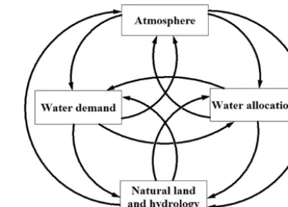
Conceptually, water resource management at larger scales can be seen as an integration of two fully interactive el-ements, related to water demand as well as water supply and allocation: water demand is constrained by water avail-ability and drives water allocation, which results in extrac-tion from water sources and determines the extent of change in hydrological elements of the land surface. Moreover, as noted briefly above, perturbations in the terrestrial water cy-cle due to water resource management can further interact with other elements of the Earth system, particularly with climate (see Fig. 1). To assess the impacts of water resource management on land-surface processes and associated feed-backs with climate, the elements of water demand and wa-ter allocation should be described using computational algo-rithms and included in large-scale models. For the purpose of our survey, and reflecting the state of algorithm develop-ment and data availability, we focus in this paper only on the representation of water demand, and in the Nazemi and Wheater (2015) on water supply and allocation. Here, we classify human water demands under two general categories, namely irrigative and irrigative, and further divide non-irrigative demands into municipal, industrial, environmental, energy-related, and livestock water needs. This is useful to put current algorithms and modeling applications into con-text. Accordingly, we discuss how these demands are char-acterized using various computational algorithms. As will be

Figure 1. Water resource management as an integration of water demand and water allocation and its interactions with natural land-surface and climate.

shown later in this paper, human demands are mainly quan-tified either using downscaling (i.e., top-down approaches) or through direct modeling at the grid scale (i.e., bottom-up approaches). Depending on the type of application, the algorithms can be included in a wide range of large-scale models. Throughout our review, we consider both offline and online implications of water demand. Offline simulations as-sess the effects of water demand on land-surface processes without considering the associated feedbacks to the climate system, but can be linked to atmospheric driving variables to simulate land-surface and/or hydrological responses to cli-mate and water resource management. Online models also account for the effects of water demand on land–atmospheric feedbacks and are further coupled with climate models. This is done by considering the effects of water demand on the dynamics of land-surface variables and updating the sur-face boundary conditions in climate models (Verseghy, 1991, 2000; Verseghy et al., 1993). Online applications are also termed in the LSM community as coupled land–atmospheric simulations (e.g., Entekhabi and Eagleson, 1989; Noilhan and Planton, 1989) and are more computationally demand-ing compared to offline simulations. While offline models in-clude both LSMs and GHMs, it should be noted that GHMs cannot be used for online applications as they do not account for the energy balance and therefore cannot fully represent land–atmosphere feedbacks.

part of our survey and outlines our main findings with respect to representing human water demand.

2 Types of human demand and their impacts on the water cycle

Human water demands can be divided into irrigative and non-irrigative categories. Irrigation is the dominant human water use and has significantly intensified since the 1950s, due to population growth and technological development (Steffen et al., 2011). This has major importance for global food secu-rity, as it produces approximately 40 % of the world’s food (Abdullah, 2006). Currently, around 25 % of harvested crop area is irrigated (Portmann et al., 2010). This accounts for some 90 % of water consumption at the global scale (Döll et al., 2009; Siebert et al., 2010), which is around 70 % of the total water withdrawals from surface and groundwa-ter resources (Wisser et al., 2008; Gerten and Rost, 2010). Clearly supplying such a large water demand can severely disturb the “natural condition” by decreasing streamflow vol-ume (e.g., Meybeck, 2003; Gaybullaev et al., 2012; Lai et al., 2014) and groundwater levels (e.g., Rodell et al., 2009; Glee-son et al., 2012; Wada et al., 2010, 2012, 2014; Döll et al., 2014). Currently, surface water is the main supplier of global irrigative needs, accounting for 57 % of the total consumptive irrigation use at the global scale (Siebert et al., 2010).

Apart from driving hydrological changes, irrigation-induced changes in soil moisture can affect land surface– atmosphere feedbacks (see Eltahir, 1998). Pokhrel et al. (2012) showed that increased soil water content through irrigation substantially enhances evapotranspiration, and therefore transforms the surface energy balance. Evapotran-spiration due to irrigation leads to cooling of the land surface (e.g., Haddeland et al., 2006; Saeed et al., 2009; Destouni et al., 2010), as well as enhanced cloud cover and chance of convective precipitation (e.g., Moore and Rojstaczer, 2001; Douglas et al., 2009; Harding and Snyder, 2012a, b; Qian et al., 2013). Irrigation may also alter regional circulation pat-terns due to temperature difference between irrigated areas and neighboring regions (e.g., DeAngelis et al., 2010; Wei et al., 2013). Over highly irrigated regions, this can mask im-portant climate change signals. Gerten et al. (2011), for in-stance, showed that the irrigation in South Asia has offset the increasing temperature in the region.

Non-irrigative water demands include municipal and in-dustrial uses, energy-related withdrawals, other agricultural uses, such as livestock, as well as designated environmen-tal water uses, which can be an important constraint on water management. Non-irrigative demands contribute a lesser portion to total human water use at the global scale. This pro-portion, however, has significant spatial variability (Vassolo and Döll, 2005; Flörke et al., 2013) as regional differences in population, income, life style and technological develop-ments can alter the extent of non-irrigative demand

signifi-cantly (e.g., Alcamo et al., 2003; Flörke and Alcamo, 2004; Hejazi et al., 2013a). However, while irrigation is predomi-nantly a consumptive water use, only a small portion of the non-irrigative withdrawal is consumptive (e.g., Hanasaki et al., 2013a). Non-irrigative withdrawals, therefore, partially or totally return to surface-water or groundwater systems with varying degrees of time lag. Still, this can considerably perturb the streamflow regime (e.g., Maybeck, 2003; Förster and Lilliestam, 2010). Non-irrigative water demands are cur-rently on a rapid incline due to growing population and in-dustrial development. This can increase water stress in both time and space (Hejazi et al. 2013a, b, c, d). As non-irrigative demands are mainly non-consumptive, they are less likely to change the energy balance and/or perturb the atmospheric moisture condition significantly and therefore they are less relevant to land–atmospheric interactions. However, chang-ing timchang-ing of flows can have significant local effects, for ex-ample on wetland inundation. Similarly, for some large-scale mining activities in which the extent of water withdrawals is considerable, the associated changes in soil moisture and land cover can be potentially relevant to land–atmospheric feedbacks. To the best of our knowledge, such online con-siderations for non-irrigative withdrawals have not yet been explored in the literature.

3 Available representations of irrigative demand in large-scale models

3.1 Framework and general procedure

Irrigated lands normally introduce heterogeneity into the computational grids of LSMs and GHMs. Such sub-grid het-erogeneity can be represented as an additional “tile”, similar to forested land, bare soil and snow cover (Polcher et al., 2011). Essentially, irrigation algorithms are required to es-timate the irrigation demand, and accordingly irrigative wa-ter use, at the grid scale. Here we refer to the irrigation de-mand as the water required for ideal crop growth in addi-tion to the available water from precipitaaddi-tion. To simulate the grid-based irrigation demand, crop type and the extent of irri-gated regions and growing seasons should be first identified. The location and area of irrigation districts and the associated crop types can be extracted from regional and global data sets (e.g., USDA, 2002, 2008; Siebert et al., 2005, 2007; Port-mann et al., 2010) and/or remotely sensed data (e.g., Ade-goke et al., 2003; Qian et al., 2013). There are two gen-eral approaches for identifying growing seasons. The choice of these options depends on the level of detail in the host model. In simpler models, where no energy-balance calcu-lation is available (i.e., GHMs), crops can grow when and where simple temperature- and precipitation-based criteria are met (e.g., Döll and Siebert, 2002). In more detailed mod-els (i.e., LSMs) the optimal growing season can be identified based on biophysical conditions of crop growth and/or soil water, canopy and energy balance conditions to estimate the cropping period that is necessary to obtain mature and op-timal plant biomass (e.g., Rost et al., 2008; Pokhrel et al., 2012). Both approaches are subject to uncertainty. On one hand, models with fixed crop calendars ignore inter-annual variability in growing seasons. On the other hand, even mod-els with fully dynamic crop growth algorithms may misrep-resent the seasonality. After the growing season is identi-fied, the irrigation demands (and under some assumptions, actual irrigation withdrawals) at each simulation time step can be calculated. A variety of top-down and bottom-up procedures are available for calculating the irrigation de-mand in large-scale models and are reviewed further be-low. If the irrigation demand is completely fulfilled, then the actual evapo(transpi)ration would be equal to crop-specific evapo(transpi)ration under standard conditions (see Allen et al., 1998). In offline applications, the irrigation rate can per-turb soil moisture content, evaporation, deep percolation and runoff in irrigated tiles (e.g., Hanasaki et al., 2008a, b; Wada et al., 2011, 2012, 2014). In online applications, the vertical vapor and heat fluxes need also to be considered. The total fluxes for each grid can be then calculated as the sum of the flux contributions from irrigated and non-irrigated portions of the grid (e.g., Haddeland et al., 2006; Pokhrel et al., 2012), and can be further introduced to climate models as coupled surface boundary conditions (e.g., Sorooshian et al., 2011; Harding and Snyder, 2012a, b).

3.2 Top-down algorithms for calculating irrigation demand

In top-down approaches, the irrigation demand is not directly calculated, but estimated based on downscaling information available at coarser scales, often at national or geopolitical scales. Such information is based on census-based invento-ries (e.g., Sacks et al., 2009) or socio-economic model out-puts (e.g., Voisin et al., 2013). Top-down approaches are highly influenced by the availability of global data on water use, such as FAO’s Information System on Water and Agri-culture (AQUASTAT; http://www.fao.org/nr/water/aquastat/ main/index.stm), which provides annual inventory data on national (and in some cases also sub-national) scales, and has been further extended to include socio-economic model outputs. An example of such a model is the Global Change Assessment Model (GCAM; Wise et al., 2009a, b; Wise and Calvin 2011), which estimates agricultural production based on socio-economic variables, from which the irrigation wa-ter use is indirectly calculated using the wawa-ter required for each crop per unit of land. Downscaling is performed mainly using land-use, technological and/or socio-economic prox-ies. There are various sources of uncertainty associated with top-down algorithms. First, both inventory and model-based products have major limitations due to their spatial and tem-poral scales as irrigation practices are highly variable within a country and a typical year. Moreover, the quality of both census and model-based products is poor. For instance, there are inconsistencies between census data and data quality varies from country to country (see Portman et al., 2010, for a detailed discussion). Also, socio-economic models widely ignore water availability constraints (Hejazi et al., 2013d). As a result, calculation of irrigation demand is mainly pursued through bottom-up schemes.

3.3 Bottom-up algorithms for calculating irrigation demand

ap-proaches adopt a variety of methods, and are heavily influ-enced by FAO’s guidelines for calculating irrigation water requirements (see Allen et al., 1998). These approaches are mainly used in GHMs, where the evapotranspiration is cal-culated for a reference crop and corrected as a function of crop type and development stage using a set of empirical co-efficients. Various methods are used to characterize the ref-erence evapotranspiration, such as FAO Penman–Monteith (Allen et al., 1998), Priestley and Taylor (1972) and modified Hargreaves (Farmer et al., 2011) to name a few (see McKen-ney and Rosenberg, 1993, for more examples). The choice of appropriate formulation for reference evapotranspiration is rather arbitrary and depends largely on the data availabil-ity as well as the level of detail supported in the host model. It should be noted that, due to the difference in estimation of evaporation, incorporating FAO’s guidelines for estima-tion irrigaestima-tion demand in LSMs can introduce inconsisten-cies with the evaporation estimated by the model at various timescales, particularly over dry regions where the irrigation is likely to occur (Polcher, 2014).

Here we briefly explain the currently available bottom-up algorithms, from the more simple to the more comprehensive algorithms, and highlight their strengths and weaknesses.

In the most simple bottom-up representations, the irriga-tion demand at every time step is the water required to bring the soil moisture at the root zone to saturation (e.g., Lobell et al., 2006; Harding and Snyder, 2012a, b), which describes an extreme demand condition and clearly overestimates the actual irrigation water requirement (Sacks et al., 2009). In a more realistic but still naïve representation, the soil mois-ture requirement during the growing season is considered to be the field capacity (e.g., Nakayama and Shankman, 2013); therefore, the irrigation water need is the water required to bring the soil moisture to field capacity. The description of the irrigation demand based on the field capacity can also overestimate the actual water requirements, as the evapora-tion often reaches potential level before the soil reaches field capacity. The threshold at which the evaporation reaches po-tential evaporation is crop-dependent, but often considered as a constant value in large-scale models. As an offline ex-ample, Hanasaki et al. (2008a) assumed that paddy and non-paddy crops require soil moisture content of 100 or 75 % of the field capacity at the root zone with constant depth at the global scale. Yoshikawa et al. (2014) later updated the as-sumption for non-paddy soil moisture requirement and used 60 % of field capacity, referring to the requirement for wheat. This is again rather unrealistic as (1) by assuming a constant percentage of the field capacity for all crop types, the diver-sity in crop water requirement is ignored; and (2) a constant root zone depth at the global scale can result in misestimat-ing the irrigation demand. There are attempts to address these limitations. For instance, Sorooshian et al. (2011) assumed that the required soil moisture content can change for each grid based on the dominant crop. Leng et al. (2013) and Qian et al. (2013) implemented root growth in their irrigation

de-mand algorithm to avoid overestimation of dede-mand due to a constant root zone. It should be noted that calculating the root growth is also subject to uncertainty; however, associ-ated limitations remain beyond the scope of this paper.

More realistic definitions of irrigation water demand are based on the difference between the crop-dependent potential evapotranspiration and available crop water. This definition has been widely used in global irrigation demand projections (see Table 2). In earlier examples (e.g., Döll and Siebert, 2002; de Rosnay et al., 2003), crop development is described by constant monthly multipliers for potential evapotranspira-tion and the effective rainfall is used as a surrogate for avail-able crop water. In more advanced algorithms, the correction factors are considered as functions of daily climate, stage of vegetation and root growth. Moreover, actual evapotranspira-tion or soil moisture content can be used instead of effective rainfall (Haddeland et al., 2006, 2007; Gueneau et al., 2012). There are two key limitations associated with this approach to simulation of irrigation demands. First, FAO’s definition of irrigation water requirement considers both transpiration from crop and evaporation from soil. It has been noted that this quantification may result in overestimating the irrigation demand and may not properly represent the dynamics of veg-etation (Polcher et al., 2011). Second, it is assumed that crop growth is a function of water availability only; therefore, the effects of other drivers such as CO2 on photosynthesis are

wholly ignored.

Some efforts try to overcome these limitations by defining irrigation demand based on potential transpiration instead of potential evapotranspiration (e.g., Wada et al., 2011, 2012), in conjunction with models that have more comprehensive vegetation schemes. Potential transpiration is the transpira-tion that would occur if the crop is not water stressed. Po-tential transpiration takes into account CO2 fertilization

ef-fects and can represent the adaptation of the plants to cli-matic conditions and/or crop growth cycles, if the host model is equipped with relevant calculations (Guimberteau et al., 2012); therefore, this approach is mainly used in LSMs with detailed consideration of vegetation growth. As an exam-ple, Rost et al. (2008) coupled a transpiration deficit algo-rithm with the Lund-Potsdam-Jena managed Land scheme (LPJmL; Bondeau et al., 2007), which has a detailed vege-tation growth module based on carbon and water availability (see Sitch et al., 2003; Gerten et al., 2004). The crop ter limitation was calculated based on the atmospheric wa-ter deficit, soil moisture, plant hydraulic states as well as the CO2effects. Considering the effects of both carbon and water

in vegetation can provide a basis for explicit linkage between CO2emission, crop growth and irrigation water requirement.

This would be important for future predictions under increas-ing CO2effects. Moreover, some recent simulations showed

po-tential transpiration algorithm depends strongly on the way various tiles are treated at the grid scale. Normally, LSMs can define multiple crops at the grid scale and can distin-guish the various water needs across different tiles within a grid. If potential transpiration is implemented consistently with sub-grid soil moisture divisions, then the water taken from the irrigated tiles optimizes photosynthesis and is only evaporated by the crops and not used by other surface types (e.g., bare soil, non-irrigated crops). In contrast, if all tiles share the same soil moisture reservoir at the grid scale, ir-rigation will increase the soil moisture and evaporation and therefore reduce water stress over the whole grid.

3.4 Projection of irrigative demand

From water and food security perspectives, particularly un-der various global change scenarios, it is crucial to investi-gate future irrigation demand and assess various possibilities for irrigation deficit. Climate model projections under IPCC emission scenarios (IPCC, 2000) have been widely used to force bottom-up irrigation demand algorithms (e.g., Ar-nell, 1999; Wada et al., 2013; Rosenzweig et al., 2014). Ef-forts have been also made to include intermediate socio-economic scenarios that can be matched to current climate change scenarios (see, e.g., Arnell, 2004; Fischer et al., 2007; Alcamo et al., 2007). For irrigation, intermediate scenar-ios describe changes in irrigated areas, irrigation efficiency and crop type, using empirical approaches. For example, Hanasaki et al. (2013a) recently proposed intermediate sce-narios based on newly developed Shared Socio-economic Pathways (SSPs; Kriegler et al., 2012; see also Moss et al., 2010), which are consistent with Representative Concentra-tion Pathways (RCPs; Meinshausen et al., 2011; K. E. Taylor et al., 2012). Constructing intermediate scenarios using em-pirical procedures, however, is uncertain as mechanisms that link irrigation expansion to socio-economic factors are not fully known and current empirical relationships can contain large uncertainties. More dynamic linkage between irrigation expansion and socio-economic drivers can be provided by coupled socio-economy–energy–carbon models. One emerg-ing model of such a kind is GCAM, which has been re-cently implemented for simulating the future expansions in irrigation areas and demands (Hejazi et al., 2013b, c, d) as well as policy implications for irrigation water requirements (e.g., Chaturvedi et al., 2013a, b). Although these models can represent the dynamic effects of various drivers on irrigation, they remain uncertain as their simulations are rather coarse and do not incorporate water availability constraints. There are emerging efforts to avoid this limitation by linking the irrigation demand to climate, economy and water manage-ment constraints. This can result in prediction of regions in which irrigation can be developed and sustained consider-ing changconsider-ing climate, water availability, water price and wa-ter management infrastructure (see Nassopoulos et al., 2008,

2012). Such approaches however have not been applied at larger regional and global scales.

4 Available representations of non-irrigative demand 4.1 Forms and drivers of non-irrigative demand Non-irrigative water demands relate to a wide range of envi-ronmental, municipal, industrial and energy-related uses, as well as other agricultural water needs (e.g., livestock), and in-clude both consumptive and non-consumptive withdrawals. Among these, livestock water demand is assumed fully con-sumptive, and can be estimated by livestock number and de-mand per livestock head (e.g., Wada et al., 2011; Strzepek et al., 2012b; Hejazi et al., 2013d). Wada et al. (2014) made a further improvement by estimating daily livestock require-ments at 0.5◦_×0.5◦ _{spatial resolution using livestock data} of Steinfeld et al. (2006). Daily demand was considered as a function of daily temperature.

In contrast to livestock water demand, environmental flow needs can be considered as a fully non-consumptive need, re-quired to protect rivers’ health and aquatic life. Considering the extent of environmental degradation at the global scale, accounting for environmental flow needs becomes more and more relevant and should be considered as an integral part of water resource management at larger scales. Tharme (2003) made an extensive review of available methodologies for es-timating environmental flow needs and identified more than 200 methodologies based on various hydrological, hydraulic rating, habitat simulation and holistic guidelines at the river basin scale. There are also some recent trends to involve scientists, water-resource managers and stakeholders to an-alyze available hydrological information and convert them into ecologically based and socially acceptable goals for es-timating the environmental flow needs (see Poff et al., 2009). Such procedures however are widely dependent on the avail-ability of relevant information and, therefore, cannot be eas-ily implemented in large-scale models. Currently, implemen-tation of environmental flow needs in large-scale models re-mains rather limited and simplistic and these needs are often calculated based on generic rules. For instance, Smakhtin et al. (2004) assigned thresholds for fair (Q90), natural (Q50)

and good (Q75) natural flow conditions. Shirakawa (2004,

2005, referenced from Hanasaki et al., 2008a) distinguished between two factors, i.e., minimum and perturbation flow re-quirements, which can also accommodate transient stream-flow conditions. Currently, the perturbation stream-flow require-ments are often ignored in large-scale models and the envi-ronmental needs are estimated as a minimum flow threshold (oftenQ90or 10 % of mean annual), which should be

with a 10-year recurrence period as the environmental flow requirement. Although these rules are easily implementable for larger regions and global scales, they widely ignore nat-ural system complexity and the local policy context and can contribute to misunderstanding of the extent of environmen-tal water stress (Arthington et al., 2006).

At this stage of model development, municipal, industrial and energy-related water demands are considered as the most dominant forms of non-irrigative uses. These demands are estimated using complex functions of socio-economic and technological factors, with high variability in time and space. Population is the most significant factor driving these with-drawals (e.g., Alcamo et al., 2003; Hanasaki et al., 2008a; Wada et al., 2014). National gross domestic product (GDP) is also a strong factor (e.g., Gleick, 1996; Cole, 2004; Wada et al., 2011). Although higher GDP may trigger more mu-nicipal water use per capita (Alcamo et al., 2007), Hughes et al. (2010) showed that, in general, water uses per capita are greater in developing than developed countries due to low-tech water delivery and industrialization. Strzepek et al. (2010) argued that industrial water use increases with the level of resource industry and decreases when a coun-try moves toward the service sector. Industrial technology is another important factor for non-irrigative use as the extent of both consumptive and non-consumptive uses can signif-icantly change based on the type of technology. Macknick et al. (2011), for instance, provided estimates of total wa-ter withdrawals and consumption for most electricity genera-tion technologies within the US. Comparing to recirculating cooling technology, they noted that once-through cooling re-quires 10 to 100 times more water withdrawal per unit of electric generation. However, the latter consumes less than half of the water consumed by recirculating cooling technol-ogy. Climate can be another important factor controlling both consumptive and non-consumptive withdrawals (e.g., Wada et al., 2011, 2014; Hejazi et al., 2013a; Voisin et al., 2013), but has often been ignored as an explicit driver of non-irrigative water demand.

4.2 Top-down algorithms for estimation of grid-based non-irrigative withdrawals

Unlike irrigation demand, top-down approaches have been widely used for non-irrigative withdrawals to transfer na-tional or geopolitical data to basin or grid scales. Various downscaling procedures have been suggested, based on dif-ferent proxies (see Table 4). These top-down schemes are heavily influenced by the availability of national and global data sets and the downscaling algorithms within the Wa-ter – Global Assessment and Prognosis scheme, which is a global water budget and use model (WaterGAP; Alcamo et al., 1997, 2003, 2007). Currently, the availability of different global information sources has provided the opportunity to generate gridded products from different sources. As an ex-ample, Hanasaki et al. (2008a) merged the FAO-AQUASTAT

data with population distributions and national boundary in-formation from Columbia University (CIAT, 2005) and the consumptive ratios of Shiklomanov (2000) to come up with gridded industrial and municipal water withdrawals and uses at the global scale. More detailed information on various in-dustrial uses resulted in breaking down the inin-dustrial with-drawals into their components. For instance, Vassolo and Döll (2005) distinguished between industrial water uses re-lated to thermoelectric power generation and manufacturing production. Temporal disaggregation of annual withdrawals, however, has received much less attention. Recently Wada et al. (2011, 2014) and Voisin et al. (2013) developed simple algorithms to disaggregate annual data to monthly and daily estimates (see Table 5).

4.3 Projection of non-irrigative demand

Characterizing the past and future evolution of non-irrigative demands is required to understand the mechanisms con-trolling water use and water allocation. Current projections have coarse temporal and spatial resolution and describe non-irrigative demands as functions of socio-economic and technological developments (e.g., Davies et al., 2013; Blanc et al., 2013; Hejazi et al., 2013b, d; Voisin et al., 2013). These changes can be characterized by intermediate socio-economic and technological scenarios, as briefly explained above for irrigation expansion (see Sect. 3.4). The projected demands can be further downscaled using various proxy vari-ables, as explained in Sect. 4.2. Table 6 summarizes some representative efforts, which can be classified as explicit and implicit algorithms. In explicit algorithms, changes in water withdrawals are directly described as functions of changes in socio-economy, technology and water price using simple parametric structures (e.g., Strzepek et al., 2012b; Flörke et al., 2013; Hanasaki et al., 2013a; Hejazi et al., 2013a). The parameters can be assigned using the available global and re-gional data. In implicit procedures, first the production (or population) is estimated based on integrated economy and population models or prescribed scenarios. By considering the amount of water withdrawal per unit of production (or population) and accounting for technological and/or socio-economic shifts, water withdrawals are consequently pro-jected.

5 State of large-scale modeling applications

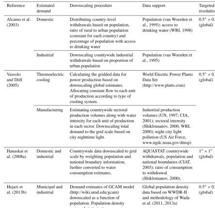
con-Table 4. Representative examples calculating grid-based non-irrigative demands using downscaling of coarse-scale estimates.

Reference Estimated Downscaling procedure Data support Targeted

demand resolution

Alcamo et al. Domestic Distributing country-level Population (van Woerden et 0.5◦×0.5◦

(2003) withdrawals based on population, al., 1995); access to (global)

ratio of rural to urban population drinking water (WRI, 1998) (constant for each country) and

percentage of population with access to drinking water

Industrial Downscaling countywide industrial Population (van Woerden et withdrawals based on proportion of al., 1995)

urban population

Vassolo Thermoelectric Calculating the gridded data for World Electric Power Plants 0.5◦×0.5◦

and Döll cooling power production based on Data Set (global)

(2005) downscaling global estimates. (http://www.platts.com)

Allocating constant flow to each unit of production according to type of cooling system.

Manufacturing Estimating countrywide sectoral Industrial production production volumes along with water volumes (UN, 1997; CIA, intensity for each unit of production 2001); sectoral intensity in each sector. Downscaling total (Shiklomanov, 2000; WRI, demand to the grid scale based on 2000); night city light city nighttime light. pollution (US Air Force,

www.ngdc.noaa.gov/dmsp)

Hanaskai et Domestic and Countrywide data downscaled to grid AQUASTAT countrywide 1◦×1◦ al. (2008a) industrial scale by weighting population and withdrawals, population and (global)

national boundary information, national boundaries (CIAT, further converted to water 2005); ratio of consumption

consumption estimates. to withdrawal

(Shiklomanov, 2000).

Hejazi et Municipal and Demand estimates of GCAM model Global population density 0.5◦×0.5◦ al. (2013b) industrial (http://wiki.umd.edu/gcam) data based on WWDR-II (global)

downscaled as a function of and methodology of Wada population. Population density et al. (2011, 2013a) assumed static in time.

Table 5. Representative examples for disaggregating annual non-irrigative demand into monthly estimates.

Reference Estimated Disaggregation procedure Data support

demand

Wada et al. Municipal Downscaling annual demand to monthly fluctuations CRU (New et al., 1999,

(2011, 2014) and livestock as a function of temperature 2000)

Voisin et al. Electrical Dividing electrical use into industry, transportation and CASCaDE

(2013) building sectors. Assuming uniform distribution for (http://cascade.wr.usgs.gov) industry and transportation uses and capturing the

ditions, and provide relatively more consistent results. Here, we briefly summarize recent applications and highlight the limitations in current simulations.

5.1 Online representation

Recent studies have shown that including irrigation in cou-pled land-surface schemes can generally improve climate simulations. With respect to regional temperature, for in-stance, Saeed et al. (2009) showed that representing irriga-tion activities over northwestern India and Pakistan can re-duce climate model simulation bias by 5◦K. It should be noted, however, that there are still large disagreements in quantifying the effects of irrigation on regional and global temperature (see, e.g., Boucher et al., 2004 vs. Lobell et al., 2006), mainly attributed to the difference in the implemented irrigation demand calculations. Sacks et al. (2009) tried to overcome the limitations in demand algorithms by down-scaling the AQUASTAT irrigative water use data to the grid scale. They concluded that irrigation has significant impor-tance for regional temperature, but at global scale the tem-perature cooling in some regions due to irrigation is can-celed by temperature warming in some other areas due to climate, land-cover and circulation changes. There are, how-ever, some limitations in their study, as the irrigation demand did not vary between years and they applied irrigation only when the LAI is around 80 % of the annual LAI. These as-sumptions can result in large uncertainty.

Irrigation-induced precipitation has been studied for quite some time and irrigation has been shown to have a sig-nificant effect on local and regional precipitation patterns (e.g., Barnston and Schickedanz, 1984; Moore and Rojs-taczer, 2001). For instance despite regional decline, Tuinen-berg et al. (2011) found a positive precipitation trend in cli-mate stations located in the irrigated regions of the south-ern Asia. Lucas-Picher et al. (2011) tested four climate mod-els and argued that lack of representation of irrigation is the main reason for precipitation bias over the Indian monsoon area. Guimberteau et al. (2012) showed that irrigation can also affect the onset of mean monsoon date over the Indian peninsula, leading to a significant decrease in precipitation during May to July. Nonetheless, there are still large dis-agreements in (1) identifying the dominant mechanisms that drive the irrigation-induced precipitation; and (2) estimating the amount and spatial extension of change in precipitation. DeAngelis et al. (2010) noted that the growing season pre-cipitation increased in the Great Plains of the US during the 20th century as a result of intensive irrigation. Using vapor tracking analysis, they indicated that evaporation from irri-gated lands adds to downwind precipitation, which increases as the evaporation increases. Harding and Snyder (2012a, b), however, noted that the extent of effects on precipitation also depend on the antecedent soil moisture. They argued that, in low soil moisture conditions, further irrigation can result in suppression of regional precipitation. Guimberteau

et al. (2012) argued that these contrasting results might be due to differences in local moisture, where the irrigation is applied. Based on a 30-year simulation, they showed an in-crease in summer precipitation over the arid western region of the Mississippi River basin in association with enhanced evapotranspiration. However, a decrease in precipitation was identified over the wet eastern part of the basin. These re-sults, however, are based on only one set of models and the coarse grid resolution might degrade the quality of simula-tions – see the discussion below. With respect to the scale of disturbance, Sorooshian et al. (2011) showed that irriga-tion over California’s Central Valley significantly decreases local temperature and increases local precipitation; however, they argued that the effects of irrigation do not expand far from the place where irrigation takes place. In contrast, Lo and Famiglietti (2013) argued that irrigation in California’s Central Valley intensifies the water cycle in the southwestern US and can increase the flow in the Colorado River.

There are two main limitations associated with available simulations of irrigation-induced rainfall discussed above. First, in most of the online studies, water availability is not a constraint. As a result, the water balance is not closed and they simply analyze whether evaporation increase can en-hance atmospheric moisture convergence or not. This can be considered as a major limitation as the available water can control the extent of irrigation (and consequently evapora-tion) and stabilize the associated feedback processes. Sec-ond, it is known that sharp landscape contrasts (i.e., transi-tions between wet and cool as well as dry and hot areas) crit-ically affect rainfall formation (e.g., Taylor 2009; C. M. Tay-lor et al., 2012). Although irrigation can create such tran-sitions due to enhanced evaporation and decreased surface temperature, current LSMs are generally unable to gener-ate the atmospheric perturbations due to these transitions (Polcher, 2014). Due to these limitations, the results of cur-rent sensitivity analyses should be considered with caution.

Online simulations under future climate change are limited and have been performed mainly at regional scales. Gerten et al. (2011) used a nested regional climate model to dy-namically downscale the future simulations of a global cli-mate model over southern Asia and considered two modes of simulation: with or without irrigation. They concluded that including irrigation can result in roughly half of the temperature increase predicted without representing irriga-tion. With respect to future precipitation, simulation with and without irrigation both showed a decrease in precipita-tion over northern India and increase in precipitaprecipita-tion over the southern peninsula; the latter was enhanced with irrigation. They noted that the increase in precipitation cannot be seen if the global-scale simulations are not dynamically down-scaled. This highlights the importance of including irrigation schemes in regional climate models for dynamic downscal-ing of future climate change scenarios.

al-gorithms and simulation settings, significant feedback ef-fects are associated with irrigation. Large uncertainties, how-ever, exist in current coupled irrigation–land-surface–climate modeling, which emphasizes the need for more research in this area.

5.2 Offline representation

Offline representation of water demands is more common, and a wide variety of GHMs and LSMs in conjunction with different demand algorithms have been used to simulate the dynamics of water demand under both current and fu-ture conditions. The available global simulations under cur-rent conditions are compared and summarized in Wada et al. (2014) and Chaturvedi et al. (2013a, b) for irrigative de-mands and in Alcamo et al. (2003) and Hejazi et al. (2013b) for total water consumption. Although incorporating water demand calculations can generally result in more realistic river discharge simulations (see Ngo-Duc et al., 2005a, b, 2007), current simulations exhibit large differences in esti-mates of water demand and use at countrywide, continental and global scales. This can be referred to the differences in data support, demand calculation schemes and host models – see the discussion of Sect. 6.

Normally, future projections of water demands include more uncertainty than simulation of current conditions as they are also conditioned on uncertain climate futures and/or socio-economic and technological scenarios. Considering fu-ture climate projections, with or without considering irriga-tion expansion, irrigairriga-tion demand algorithms have mainly projected increase in irrigation demand under climate change scenarios. As an early example, Fischer et al. (2007) es-timated irrigation water requirement as a function of both projected irrigated land and climate change from 1990 to 2080. They showed that the impact of climate change on increasing irrigation water requirement could be nearly as large as the changes initiated by socio-economic develop-ments. There are, however, two sets of uncertainty associated with future projections of irrigation demand. First, gridded climate products have significant deficiencies in representing current and future climate, particularly with respect to pre-cipitation (e.g., Lorenz and Kunstmann, 2012; Grey et al., 2013). This can further propagate to estimation of irrigation demand at the sub-grid scale. Second, there are large dis-agreements between irrigation demand projections with re-spect to different climate model simulation, irrigation algo-rithms and host large-scale models. One possible approach to account for these uncertainties would be using a multi-model approach, as recommended by Gosling et al. (2011) and Had-deland et al. (2011, 2014) and implemented to some extent by Wada et al. (2013) and Rosenzweig et al. (2014). Based on the latest IPCC climate scenarios (K. E. Taylor et al., 2012), these studies generally concluded that a significant increase in future demand is likely, with possibly 1-month or more shift in the peak irrigation demand in mid-latitude regions

(Wada et al., 2013), but large uncertainties are associated with the predictions (see Rosenzweig et al., 2014). Moreover, both studies noted that CO2increases might have beneficial

effects on crop transpiration efficiency, if other factors are not limiting (see also Gerten et al., 2011; Konzmann et al., 2013). Nonetheless, it still remains unclear whether increased tran-spiration efficiency is canceled out by increased trantran-spiration due to increasing biomass and plant growth. More studies, therefore, are required in this direction (see Gerten, 2013). This is a context for which LSMs can offer an ideal platform as they have the explicit modules required for considering dynamic interactions of carbon, vegetation and water – see the discussion of Sect. 6.

Similar conclusions were obtained with respect to non-irrigative demands. Alcamo et al. (2007) and Hejazi et al. (2013d) showed that increasing domestic and industrial water uses, if not controlled, can be a major threat for water supply. There are, however, large discrepancies between dif-ferent projections of non-irrigative demands (Gleick, 2003), in which the divergence between modeling results becomes more highlighted as the projection horizon increases (see Davis et al. (2013) for electrical demand and associated wa-ter use). These uncertainties can be referred to limitations in current data availability for supporting robust and reliable projections, differences in socio-economic and technologi-cal scenarios, as well as some underlying assumptions in de-mand calculation algorithms, which can limit their efficiency in future simulations.

As the current global potential for expanding water de-mand is rather limited (Rost et al., 2009; Gerten and Rost, 2010), adaptation and mitigation strategies are required to moderate human water demands. In such cases prescribed “policy” scenarios can be introduced into large-scale mod-els for impact assessment. Using this approach, it has been shown that mitigation can significantly decrease future global water demand. For example, Hanasaki et al. (2013a) showed approximately 7-fold and 2.5-fold variation in in-dustrial and municipal demands, depending on the SSP con-sidered. The effects of mitigation, however, have large re-gional variation. For irrigative demands, Fischer et al. (2007) showed that some regions may be negatively affected by mitigation actions, which depend on specific combinations of CO2 changes that affect crop water requirement and

projected precipitation and temperature changes. Kyle et al. (2013) showed that applying CO2mitigation policies can

are employed. Large-scale models also showed that promot-ing international trade can be a strong adaptation option for controlling regional demand, in which water-limited re-gions can import water-expensive products from other areas (e.g., Siebert and Döll, 2010; Hanasaki et al., 2010; Konar et al., 2013). Assessment of trade scenarios and water foot-printing, however, needs detailed tracking of the water cycle (see Chenoweth et al., 2014) and is highly dependent on how reasonable the human demands and production, as well as water availability and water allocation, are described in time and space. Such a level of accuracy is currently not available and therefore the assessments remain widely uncertain.

In summary, current offline projections agree on large im-pacts of future change in climate, socio-economy and tech-nology on water demands and the importance of adaptation and mitigation strategies for managing future water security threats. Available projections, however, are rather limited and suffer from major sources of uncertainty, which is revealed by large discrepancies between different simulation products under current and future conditions. We now turn to discuss these gaps in more detail and identify the research needs and priorities.

6 Discussion

Major gaps remain in the current capability in modeling wa-ter demands and understanding their online and offline im-pacts on the terrestrial water cycle and human livelihoods. These gaps are partially due to inherent complexity in model-ing Earth system processes, which is more significant in cou-pled simulation modes. Apart from various computational barriers, one main challenge in online simulations is the uncertainty associated with coupling land and atmospheric models, as given a unique land-surface boundary condition, the simulations obtained by different climate models can be divergent (Koster et al., 2004; Pitman et al., 2009; Dadson et al., 2013). Another major challenge for coupled irrigation– land-surface–climate simulations is the choice of appropri-ate temporal and spatial resolutions, at which the relevant physical processes and feedbacks between land and atmo-sphere should be represented and described. Ideally, the opti-mal modeling resolution should be identified based on phys-ical realism; nonetheless, the choice of resolution in cou-pled simulations is mainly constrained by computational re-sources, data availability and the complexity supported by the LSMs. If these are not limiting factors, it has been shown that finer temporal and spatial resolutions can improve online representation of irrigation. For instance, using six differ-ent combinations of temporal/spatial resolutions, Sorooshian et al. (2011) concluded that spatial and temporal resolution in coupled irrigation–land–climate models can significantly change both temperature and precipitation simulations over irrigated grids and a fine level of detail is required for rep-resenting the physical processes controlling the feedbacks

between irrigation and atmosphere. However, these findings remain regionally and seasonally dependent and are closely linked to the level of complexity supported in the consid-ered irrigation parameterization and host model. It should be noted that, by increasing the spatial resolution, more pro-cesses need to be included in order to ensure water conser-vation within the model and that can further complicate the issues related to water availability – see the discussion below. The effects of fine modeling resolution seem to be in general less significant in offline runs, as far as the evaporation cal-culation is consistent with estimation of crop water require-ments and each crop is supplied by a unique moisture reser-voir. Compton and Best (2011) conducted offline global sulations and showed that fine spatial resolution has little im-portance on long-term modeling of evaporation and runoff; however, the temporal resolution does change the mean evap-oration/runoff balance. The issues around modeling resolu-tion are explored further in Nazemi and Wheater (2015).

Large uncertainties are also associated with offline human water demand simulations under current and future condi-tions. Lissner et al. (2012), for instance, noticed significant difference in terms of water demand per capita between the simulated products of WaterGAP and reported AQUASTAT data. These uncertainties are mainly related to (i) available data support, (ii) demand calculation algorithms and (iii) host models. These sources are widely connected and cannot be easily addressed and quantified independently. Here we briefly discuss these sources and propose few directions for future developments.

This can be important for understanding the amount of water loss and thus estimating the actual irrigation use and evaporation (see, e.g., Evan and Zaitchik, 2008). The issues around data support apply to non-irrigative demands as well. For the case of water use for electricity generation in the US, Macknick et al. (2011) noted that “federal data sets on water use in power plants have nu-merous gaps and methodological inconsistencies.” Data uncertainty can propagate into structural and parametric identification during model development and can fur-ther extend to future projections. The availability of dif-ferent sources of global and regional data has resulted in emergence of various data sets, with varying degrees of quality, which can potentially support demand calcu-lation algorithms. At this stage of research, the various data sets have not been systematically compared with respect to their uncertainty and the associated effects on demand simulations. This is a major need for future ex-ploration.

2. Uncertainty in demand calculation algorithms: this in-cludes both irrigative and non-irrigative demands.

a. Irrigative demand: limitations in current algorithms mainly include the uncertainty in describing the crop moisture requirements in time and space and constraining the irrigation to water availability. If the irrigation is limited by the water available at the grid scale, then the quality of simulation is hin-dered by the ability of the host model to describe water allocation from surface and groundwater re-sources (see Nazemi and Wheater, 2015). In addi-tion, current bottom-up algorithms do not appropri-ately consider plant-specific water requirements at the sub-grid scale due to missing soil and crop di-versity. This can result in misestimating the irriga-tion demand. In the best situairriga-tion, where the same assumption is used for the calculation of the crop evaporation and the irrigation demand, the uncer-tainty of the irrigative demand is the same as evap-oration, but this can still vary greatly across var-ious host models. Considering future simulations, widely used irrigation demand estimates based on FAO guidelines often require several input vari-ables (see, e.g., Farmer et al., 2011 and Hejazi et al., 2013b, for simplifications), and given the need for downscaling of climate variables for future simula-tions, these can be outperformed by simpler models (e.g., Vörösmarty et al., 1998; Wisser et al., 2010). At the current stage of research, different meth-ods for calculating irrigative demand have not yet been fully intercompared to identify appropriate al-gorithms with respect to region, climate and type of crops. This can be considered as an important need for further research. Another avenue for future de-velopment is improving the demand simulations

us-ing data assimilation and model calibration. These opportunities will be discussed further in Nazemi and Wheater (2015).

b. Non-irrigative demand: the current offline model-ing capability is generally temporally coarse, and available downscaling and projection algorithms mainly do not account for seasonal variations in water demand. There are also parametric and struc-tural uncertainties in functional mappings that link water demand to socio-economic and technologi-cal proxies due to limitations in available data as well as the diversity and spatiotemporal variabil-ity in non-irrigative demands. At this stage, it is not fully understood how these uncertainties propa-gate into future projections considering additional uncertainty in future climate and socio-economic scenarios. Developing robust downscaling and pro-jection algorithms for estimation of non-irrigative demands therefore is an important need for future development.

3. Uncertainty in host models: host models can add sub-stantial uncertainty to demand simulations, particularly for irrigation. As noted in Sect. 3, the calculation of ir-rigation demand involves solving the soil water balance at every simulation time step and this is determined by how the relevant natural processes, such as actual evap-otranspiration and soil moisture, are parameterized in the host model. Haddeland et al. (2011) showed major differences in the global simulations obtained from six LSMs and five GHMs due to differences in underlying assumptions, process representations, and related pa-rameterizations. It is also shown that considering feed-back effects between irrigation and atmosphere can con-siderably change potential evaporation (e.g., Blyth and Jacobs, 2011; Lu, 2013); therefore offline irrigation de-mand simulations based on GHMs might be biased as they inherently ignore climate feedbacks. Moreover, GHMs often cannot represent important processes such as the effects of increased carbon concentration on ir-rigation demand. This limitation may result in major deficiencies in simulating climate change scenarios as CO2 increases can significantly change vegetation

dy-namics (e.g., Prudhomme et al., 2014), which can fur-ther alter the evaporation and runoff regimes (Gerten et al., 2004). From this perspective, it can be concluded that online LSMs are superior to GHMs with respect to simulations under increasing CO2concentration and