Interannual to multidecadal hydroclimate variability and its sectoral impacts in northeastern Argentina

https://doi.org/10.5194/hess-22-3155-2018 © Author(s) 2018. This work is distributed under the Creative Commons Attribution 4.0 License.

Interannual-to-multidecadal hydroclimate variability and its

sectoral impacts in northeastern Argentina

Miguel A. Lovino1,2, Omar V. Müller1,2, Gabriela V. Müller1,2, Leandro C. Sgroi2, and Walter E. Baethgen3

1_{Consejo Nacional de Investigaciones Científicas y Técnicas (CONICET), Buenos Aires, Argentina}

2_{Centro de Estudios de Variabilidad y Cambio Climático (CEVARCAM), Facultad de Ingeniería y Ciencias Hídricas,}

Universidad Nacional del Litoral, Santa Fe, Argentina

3_{International Research Institute for Climate and Society, Columbia University, Palisades, USA}

Correspondence:Miguel A. Lovino ([email protected]) Received: 5 January 2018 – Discussion started: 24 January 2018

Revised: 11 May 2018 – Accepted: 18 May 2018 – Published: 6 June 2018

Abstract. This study examines the joint variability of pre-cipitation, river streamflow and temperature over northeast-ern Argentina; advances the understanding of their links with global SST forcing; and discusses their impacts on water re-sources, agriculture and human settlements. The leading pat-terns of variability, and their nonlinear trends and cycles are identified by means of a principal component analysis (PCA) complemented with a singular spectrum analysis (SSA). In-terannual hydroclimatic variability centers on two broad fre-quency bands: one of 2.5–6.5 years corresponding to El Niño Southern Oscillation (ENSO) periodicities and the second of about 9 years. The higher frequencies of the precipita-tion variability (2.5–4 years) favored extreme events after 2000, even during moderate extreme phases of the ENSO. Minimum temperature is correlated with ENSO with a main frequency close to 3 years. Maximum temperature time se-ries correlate well with SST variability over the South At-lantic, Indian and Pacific oceans with a 9-year frequency. Interdecadal variability is characterized by low-frequency trends and multidecadal oscillations that have induced a tran-sition from dryer and cooler climate to wetter and warmer decades starting in the mid-twentieth century. The Paraná River streamflow is influenced by North and South Atlantic SSTs with bidecadal periodicities.

The hydroclimate variability at all timescales had signif-icant sectoral impacts. Frequent wet events between 1970 and 2005 favored floods that affected agricultural and live-stock productivity and forced population displacements. On the other hand, agricultural droughts resulted in soil mois-ture deficits that affected crops at critical growth stages.

Hy-drological droughts affected surface water resources, caus-ing water and food scarcity and stresscaus-ing the capacity for hydropower generation. Lastly, increases in minimum tem-perature reduced wheat and barley yields.

1 Introduction

Hydroclimate variability affects natural and human sys-tems worldwide. Climate-related extremes such as droughts, floods, and heat waves alter ecosystems, disrupt food pro-duction and water supply, damage human settlements and cause morbidity and mortality (Field et al., 2014). Exam-ples around the world include annual losses of about USD 6– 8 billion to the US economy due to drought (Carter et al., 2008), and the extraordinarily severe heat wave over west-ern and central Europe in the summer of 2003 that caused about 35 000 deaths (Kosatsky, 2005), with estimated eco-nomic losses for the agriculture sector in the European Union at EUR 13 billion (Sénat, 2004).

ex-tended and persistent drought of 2008–2009 caused losses of about 40 % of grain production in Argentina and greatly af-fected the hydroelectric sector over SESA (Bidegain, 2009). The severe drought in 2011–2012 caused economic losses of USD 2.5 billion in crop production of soybean and corn in Argentina (Webber, 2012). In this context, studies in re-cent years have been focusing on understanding the impacts of the regional climate (e.g., Magrin et al., 2014 and refer-ences therein; Barros et al., 2015 and referrefer-ences therein). An-other group of studies analyzed strategies to increase the re-silience of the affected populations (Hernandez et al., 2015; Mussetta et al., 2016). Nevertheless, it is necessary a joint view of the main hydroclimatic variables and their sectoral impacts at different timescales to provide accurate and inte-grated information that will facilitate decision-making pro-cesses.

Hydroclimate in SESA varies on interannual to multi-decadal timescales. On interannual timescales, the El Niño Southern Oscillation (ENSO) is the major source of hydro-climate variability (Garreaud et al., 2009; Baethgen and God-dard, 2013). El Niño conditions can cause increased severe precipitation and streamflow while La Niña events may favor droughts (Grimm et al., 2000; Camilloni and Barros, 2003; Penalba and Rivera, 2016). Precipitation and Paraná River flow present oscillations of 3 to 6 years linked to the ENSO and a near-decadal cycle related with the North Atlantic Os-cillation (NAO) (Robertson and Mechoso, 1998; Krepper and García, 2004; Antico et al., 2014). Regarding temperature, the interannual variability modes of extreme temperature fre-quencies concentrated on a 2–4-year band and an 8-year sig-nal mostly associated with the Southern Annular Mode (Bar-rucand et al., 2008; Loikith et al., 2017).

On decadal-to-multidecadal timescales, the Pacific decadal variability (PDV) also modulates SESA hydrocli-mate in the same way as ENSO, i.e., positive SST anomalies might favor wetter conditions while negative SST anomalies might favor drier conditions (Andreoli and Kayano, 2005). Further, there are other sources of hydroclimate variability such as the Atlantic Ocean and the South Atlantic Conver-gence Zone (SACZ) (Seager et al., 2010; Mo and Berbery, 2011; Grimm and Saboia, 2015; Grimm et al., 2016). For example, the Paraná streamflow is dominated by a nearly bidecadal oscillation related to the SACZ and a multidecadal cycle forced by PDV (Antico et al., 2014).

Hydroclimate trends have been observed over SESA. Ex-treme precipitation and temperature events registered long-term increases since the 1960s as well as Paraná River flow after the mid-1970s (Haylock et al., 2006; Seneviratne et al., 2012; Cavalcanti et al., 2015; Carril et al., 2016; Scardilli et al., 2017). Huang et al. (2005) and Jaques-Coper and Gar-reaud (2015) have suggested that those changes were influ-enced by interdecadal variability in tropical Pacific SSTs. However, the wet trend in precipitation could also be favored by a multidecadal cooling in the tropical Atlantic Ocean (Seager et al., 2010; Barreiro et al., 2014).

This study has three main purposes: first, to reassess the joint variability from interannual to multidecadal scales of precipitation, streamflow and temperatures (maximum and minimum) over northeastern Argentina; second, to review and discuss the links between those hydroclimatic variables at regional scale and global SST forcing; and lastly, to dis-cuss the impacts of trends and hydroclimate variability at different timescales on water resources, agriculture and hu-man settlements. In order to fulfil these objectives, we ex-amined century-long datasets of precipitation, river flow, air temperature and SST using multivariate statistical methods to describe and characterize the historic regional hydrocli-mate variability. We also explored the relationship between leading modes of global SST variability patterns and signif-icant modes of hydroclimatic variables. Finally, we explore the impacts of hydroclimatic extremes and discuss how vari-ability at different timescales affects each sector. This pa-per reports novel findings regarding variability modes and their SST forcing factors that influence the formation of ex-treme events. It also provides an integrated and comprehen-sive discussion on the sectoral impacts of variability at dif-ferent timescales that can contribute to the identification of actions and policies for increasing the resilience of regional populations and their capacity to better cope with extreme events.

2 Methodology 2.1 Study region

The study region is located in southeastern South Amer-ica, covering La Plata Basin (Fig. 1a), which has four ma-jor subbasins: Uruguay, Paraguay, Mid–Upper Paraná and Lower Paraná (see Fig. 1b). The Paraguay and Mid–Upper Paraná subbasins contribute a high percentage of the Paraná River flow. The Lower Paraná River extends over a flat plain, where high discharges easily cause severe floods (Coronel and Menéndez, 2006). A large portion of the Lower Paraná subbasin is covered by the study region in northeastern Ar-gentina (NEA), delimited by 36–26◦S and 65–58◦W (red box in Fig. 1b). This region is key for the socioeconomic de-velopment of the country and the continent. It contains most of the country’s population, has a complex system of water resources management and produces 80 % of the cereal crop in Argentina (Ministry of Agroindustry, 2017).

2.2 Datasets

Figure 1. (a)South America and the domains of the La Plata Basin (bold black contour) and southeastern South America (blue polygon).

(b) Topography map of La Plata Basin and its subbasins (black contours), Paraguay (PAY), Mid–Upper Paraná (MUP), Lower Paraná (LOP) and Uruguay (URU). The rivers and their tributaries are plotted in blue contours. Gauging stations of the Paraná River streamflow in Corrientes (Qco) and Timbúes (Qti) are highlighted. The study area in northeastern Argentina is highlighted with a red rectangle.

According to Lovino (2015), GPCC v7 has lower biases and fits extreme fluctuations better than other precipitation datasets over the study region. While there are areas in SESA with poor rain gauge coverage, northeastern Argentina has a reasonable station distribution for the whole period (Barreiro et al., 2014).

Monthly streamflow along the Paraná River is measured at two locations: the Corrientes and Timbúes gauging sta-tions (Fig. 1b). These observed streamflow data might in-clude variations due to anthropogenic influence, particu-larly damming. The Corrientes station represents most of the Paraná basin discharge since the main tributaries are upstream (Camilloni and Barros, 2000; Berbery and Bar-ros, 2002). Corrientes station data cover from January 1904 to August 2014 with no missing values. Timbúes is fur-ther downstream and reflects precipitation variability in the Lower Paraná basin. Timbúes station data extend from September 1905 to August 2014 with only four missing val-ues that were linearly interpolated to have a continuous se-ries. All data were obtained from the Integrated Hydrologi-cal Data Base of the National Water Information System of Argentina (NWIS, 2016).

Monthly time series of the daily maximum and minimum temperatures used were obtained from the Climatic Research Unit (CRU TS 3.23, Harris et al., 2014; University of East Anglia Climatic Research Unit, 2017). The CRU dataset has a resolution of 0.5◦×0.5◦ degrees and covers the period 1901–2014. CRU TS 3.23 also fits well observed mean and extremes temperatures throughout NEA (see Lovino, 2015). Lastly, monthly SST data are those from the Extended Re-constructed Sea Surface Temperature Version 4 (ERSSTv4, Huang et al., 2015; Liu et al., 2015). The ERSSTv4 dataset is available on a global 2◦×2◦grid since January 1854.

Historical journalistic information was collected to doc-ument the impacts of the key cases of extreme events re-lated to hydroclimatic variability. We also compiled and ana-lyzed the scientific literature regarding the potential impacts of droughts, floods and heat waves over southeastern South America. The changes and variability of the regional precip-itation, flows and temperature were identified and then used as input variables to determine their joint sectoral impacts.

2.3 Statistical approach

The present analysis focuses on precipitation, streamflow and temperature (minimum and maximum) of the NEA, consid-ering SSTs as the main external forcing. For these four vari-ables, monthly mean anomalies are computed by removing the corresponding mean annual cycle. The variables are also filtered applying low-pass Lanczos filters (Duchon, 1979) with 36 weights and cut-off periods at 18 and 120 months to emphasize the interannual and low-frequency behavior re-spectively. The Lanczos filter is quite simple and yields a better response than other filters such as a running-mean ter (Duchon and Hale, 2012); for example, the Lanczos fil-ter reduces the amplitude of the Gibbs oscillation and allows the cut-off frequencies to be controlled independently of the number of weights (Duchon, 1979; Navarra, 1999).

we opted not to do it because in our case it led to patterns overly localized in space, i.e., several EOFs concentrate in-formation of the spatial patterns in small regions, hindering their interpretation (not shown; see Deser et al., 2010).

A singular spectrum analysis (SSA, Ghil et al., 2001) is then used to study the temporal variability of (1) leading PCs of precipitation and SST, (2) streamflow time series, and (3) temperature anomalies time series. SSA determines the structures of deterministic signals as nonlinear trends and quasi-oscillatory modes. In the SSA method, the win-dow lengthMshould not exceedM=N/3, whereN is the length of the time series, to adequately represent quasi-cycles betweenM/5 andM (Von Storch and Navarra, 1995). For decadal-to-multidecadal variability, we considered a window length that retains variability of the 120-month low-pass-filtered series between 10 and 30 years (M=360 months or 30 years; M/5 < 120 months or 10 years of the low-pass filter). For interannual variability, we considered a win-dow length that retain variability of the 18-month low-pass-filtered series between 2 and 10 years (M=120 months or 10 years andM/5=24 months or 2 years).

Sectoral impacts of hydroclimatic variability are evaluated at different timescales. First, we identify the key character-istic of the regional hydroclimate variability on interannual-to-multidecadal timescales and the influence of global SST forcing. Changes in precipitation, streamflow and tempera-ture are studied by nonlinear trends. Then, we address how the main properties of the variability (including extreme events) and changes affect water resources, agriculture and human settlements. Finally, we discuss the sectoral impacts attributed to hydroclimate variability by analyzing some key cases and reviewing the information available in the scientific literature.

3 Leading patterns of global SST variability

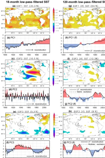
The patterns of global SSTs have been widely studied and evaluated in different timescales and periods (e.g., Schubert et al., 2009; Deser et al., 2010; Messié and Chavez, 2011). Other studies have discussed the mechanisms by which the SST patterns affect SESA hydroclimate (e.g., Grimm et al., 2000 and Seager et al., 2010 among many others). Our main interest is in discussing the leading modes of global SST variability and examining their links to significant modes of hydroclimatic variables in NEA as a necessary step to un-derstand their sectoral impacts. Figure 2 presents the three leading EOFs and their corresponding PCs of 18- and 120-month low-pass-filtered 120-monthly mean global SST fields. The three main patterns explain more than 50 and 70 % of the total variance of global 18- and 120-month filtered SSTs fields, respectively. The global SST patterns are very similar to those obtained by Schubert et al. (2009) using annual mean SSTs. Slight differences result from using monthly data in-stead of yearly data, and because the rotation was not done.

Table 1 presents the dominant modes of interannual and low-frequency SST variability for each PC.

The first pattern of 18-month low-pass-filtered global SST (Fig. 2a) displays positive loadings in most of the world ocean. The first EOF presents the highest positive loadings in the South Atlantic and the Indian Ocean, congruent with the results of Schubert et al. (2009). Also, high positive loadings are shown in the central Pacific Ocean. The first PC (Fig. 2b) is driven by a low-frequency nonlinear trend, but interannual timescales also influence PC1 with periodicities of roughly 9 and 3 years that explain 9 % of its variance (see Table 1 and the interannual reconstruction in Fig. 2b).

The second pattern (Fig. 2c) reveals a pan-Pacific pattern resembling features of the ENSO. The EOF2 displays posi-tive loadings from the central to the eastern Pacific and neg-ative values in the North and South Pacific. The spectral de-composition of the corresponding PC2 presented in Table 1 shows dominant modes at interannual timescales between 2.8 and 5.7 years. The PC2 shown in Fig. 2d has correlations of about 0.9 with indices of ENSO evolution.

The third pattern (Fig. 2e) presents positive loadings in the North Atlantic Ocean and negative loadings south of 40– 50◦S, with centers in the South Atlantic and Indian oceans. The PC3 (Fig. 4f) is mostly driven by a multidecadal oscilla-tion. The interannual variability exerts a slight effect through a cycle of approximately 4 years that represents only 3 % of the PC1 variance (see Table 1 and the interannual reconstruc-tion in Fig. 4f).

Decadal-to-multidecadal SST variability is characterized by the 120-month low-pass-filtered SST patterns (right col-umn Fig. 2). The first pattern (Fig. 2g) displays the high-est positive loading in the south Atlantic and Indian Ocean but not in the central Pacific Ocean as is the case with the EOF1 in Fig. 2a. The PC1 (lf) (Fig. 2h) exhibits a nonlinear trend that explains more than 85 % of its variance. The trend denotes an increase in global SSTs over the whole period, reaching positive anomalies since the 1960s.

The second pattern (Fig. 2i) resembles features of the Pa-cific Decadal Oscillation. Weakly positive loadings are also shown in the central and southwest Pacific Ocean and neg-ative loadings towards the North Atlantic Ocean. PC2 (lf) presents two cycles, one close to 15 years, and a multi-decadal oscillation of very low frequency (Table 1). Although the multidecadal oscillation presents periodicities out of the range that can be estimated by SSA, the spectral analysis allows us to infer periodicities of around 70 years. These decadal-to-multidecadal periodicities exhibit in Fig. 2j are positively correlated to the ones of the Decadal and Inter-decadal Pacific oscillations (as identified by Mantua and Hare, 2002 and Henley et al., 2015 respectively).

dom-Figure 2.First three leading global pattern of 18- and 120-month low-pass-filtered monthly mean SST between January 1901 and Septem-ber 2012. Patterns are described by the spatial loadings (EOFs) and their associated PCs. The percentage of variance explained by each pattern is given in brackets. The original time series are partially reconstructed using the significant components detected with SSA. Partial reconstructions at interannual timescales are plotted in PCs of the left column (IA reconstruction). Partial reconstructions at low-frequency timescales (LF reconstruction) are plotted in PCs (lf) of the right column. The partial reconstructions include all variability modes at each timescale shown in Table 1. Panels(j)and(l)also show the multidecadal oscillations.

inant frequency of the multidecadal oscillation is out of range but it seems to be about 70 years. Schlesinger and Ra-mankutty (1994) among others have reported a similar os-cillation with the same frequency in the North Atlantic. On

Table 1.Trends and dominant periodicities obtained from applying SSA to the first three PCs and PCs (lf) of the 18- and 120-month low-pass-filtered SST global patterns, respectively. The analysis is performed on interannual timescales (between 2 and 10 years) and lower frequency or decadal-to-multidecadal timescales (higher than 10 years). The percentage of variance explained by each mode is given in brackets.

Sea surface temperature

Timescale PC1 (Var) PC2 (Var) PC3 (Var)

Interannual 2.8 (10)

(18-month low-pass 3.5 (3) 3.5 (17) 4.3 (3)

filtered time series) 5.7 (32)

9.3 (6)

PC1 (lf) (Var) PC2 (lf) (Var) PC3 (lf) (Var)

Decadal-to-multidecadal 14 (8)

(120-month low-pass 20–26 (5) 13–15 (10) 20–27 (20)

filtered time series) Trend (87) Multidecadal oscillation (75) Multidecadal oscillation (67)

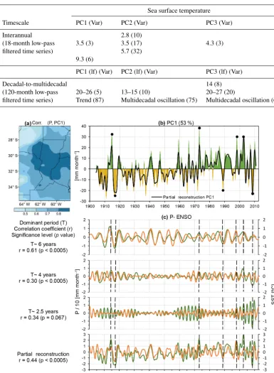
Figure 3.First leading pattern of the 18 m low-pass-filtered precipitation anomalies. Panel(a)shows the spatial distribution of the correlation between PC1 (inb) and each precipitation time series at a single grid point. The percentage of explained variance is given in brackets. Panel

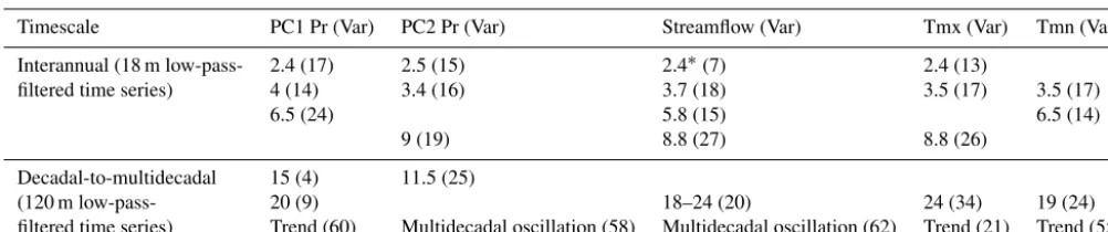
Table 2.Leading frequencies (in years) of regional precipitation patterns, monthly mean streamflow of the Paraná River, and area-averaged maximum and minimum temperature (Tmx and Tmn). Precipitation is represented by the two leading patterns of the PCA for both 18-and 120-month filtered fields. All streamflow modes were noted in Corrientes 18-and Timbúes gauging stations, except the near-biannual cycle (∗) that is only shown in Timbúes. The percentage of variance explained by each mode is given in parentheses.

Timescale PC1 Pr (Var) PC2 Pr (Var) Streamflow (Var) Tmx (Var) Tmn (Var)

Interannual (18 m low-pass- 2.4 (17) 2.5 (15) 2.4∗(7) 2.4 (13)

filtered time series) 4 (14) 3.4 (16) 3.7 (18) 3.5 (17) 3.5 (17)

6.5 (24) 5.8 (15) 6.5 (14)

9 (19) 8.8 (27) 8.8 (26)

Decadal-to-multidecadal 15 (4) 11.5 (25)

(120 m low-pass- 20 (9) 18–24 (20) 24 (34) 19 (24)

filtered time series) Trend (60) Multidecadal oscillation (58) Multidecadal oscillation (62) Trend (21) Trend (55)

4 Regional hydroclimate variability and its links to global SSTs forcing

The precipitation, streamflow and temperature over NEA exhibit spectral peaks on interannual and decadal-to-multidecadal timescales that are summarized in Table 2. On interannual timescales, hydroclimate variability centers on two bands: one with frequencies between 2.5 and 6.5 years and the other with periodicities close to 9 years. For each variable, interannual modes represent more than 50 % of their temporal variability, except for minimum temperature, which modes explain 30 % of its variance. On decadal-to-multidecadal timescales, nonlinear trends and decadal-to-multidecadal oscillations account for most of the variability, while the in-terdecadal modes (about 11–25 years) have a lesser effect.

4.1 Interannual modes

Figure 3a and b show the spatial pattern and temporal evo-lution of the first principal component of precipitation. The pattern is mainly located towards the center-east of NEA with variability within the higher interannual band (2.5– 6.5 years). Figure 3c shows that the bands of variability of the precipitation correspond to the frequencies of the ENSO-like SST pattern. This relationship is well known and has been studied in several previous works (e.g., Grimm et al., 2000; Paegle and Mo, 2002; Garreaud et al., 2009). Figure 3c shows that all the main frequencies of the ENSO (i.e., 6, 4 and 2.5 years) are also replicated in the regional precipitation, in agreement with Penalba and Vargas (2004) and Garreaud et al. (2009). The 6-year frequencies present the highest corre-lation values (r∼0.61, significant at the 99.9 % confidence level) between ENSO and regional precipitation, while the other frequencies have correlations of about 0.3. The second leading pattern of precipitation (not shown, 11 % of the to-tal variance) is located toward the northwest of NEA. The PC2 presents cycles with periodicities of nearly 3 years and within the lower interannual band of 9 years (see Table 2).

Interannual variability of precipitation has a close relation with extreme events (see the dots in Fig. 3b). In agreement

with Grimm et al. (2000) and Grimm and Tedeschi (2009), Fig. 3b and c show that some of the largest extreme precipita-tion events occurred during extreme ENSO years, including wet extreme events in 1914, 1972–1973 and 1997–1998 and severe droughts in 1916–1917 and 1988–1989. During those events, SST and precipitation cycles were mostly in phase and with high amplitudes (Fig. 3c). However, the ENSO phenomenon by itself is not enough to explain the inten-sity of the droughts and wet events. First, extreme precipi-tation anomalies were recorded during the 2002–2003 mod-erate El Niño event, and conversely, the 2008–2009 intense drought occurred under moderate La Niña conditions. Stud-ies have shown that other ocean forcing, such as the SST over the North Tropical Atlantic Ocean or the South Atlantic Convergence Zone, can combine with ENSO to intensify the wet or dry signals in precipitation, leading to extreme events (Robertson and Mechoso, 2000; Seager et al., 2010; Mo and Berbery, 2011). Second, the precipitation for the 2.5- to 4-year periods exhibits a large increase in amplitude after 2000, as noted in the mid-panels in Fig. 3c. Yet, ENSO-like SST cycles were weakened for the same period. Thus, our results suggest that interannual precipitation variability with period-icities between 2.5 and 4 years contribute to the exacerba-tion of extreme events such as those of the 2000s, even dur-ing moderate extreme phases of the ENSO. This difference could be explained by an increase in heavy rainfall resulting from greater atmospheric instability and water vapor content (see e.g. Re and Barros, 2009; Penalba and Robledo, 2010). Moreover, these intense precipitation events are strongly in-fluenced by cycles between 2 and 4 years (Lovino et al., 2018).

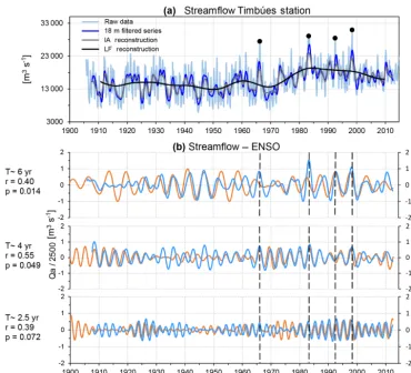
Figure 4. (a)Monthly mean streamflow time series for the Paraná River at Timbúes station and its partial reconstruction using all significant modes of interannual (IA reconstruction) and decadal-to-multidecadal variability (LF reconstruction) presented in Table 2.(b)Time series of the dominant modes of Paraná River streamflow anomalies and the ENSO pattern on interannual timescales. Streamflow modes have been scaled to facilitate their interpretation. Dominant periods (T) of the leading modes and Pearson correlation coefficients (r) together with their significance levels (p) are given to the left of the figure. Significance levels (pvalues) forrare estimated by combining 2000 Monte Carlo iterations considering autocorrelation by resampling in the frequency domain (Macias-Fauria et al., 2012). Vertical dashed lines coincide with extreme flood events in 1966, 1983, 1992 and 1998.

correspond to the ENSO-range SST periodicities (Fig. 4b), in agreement with Robertson and Mechoso (1998) and An-tico et al. (2014). We find that the 4-year cycles of ENSO and streamflow reach the largest correlation (r∼0.55, significant at the 95 % confidence level), as they are in phase for al-most the entire period (mid-panel, Fig. 4b). Cycles of roughly 2.5 years do not exhibit a strong correlation for the earlier pe-riod but become in phase mainly starting around 1980 (bot-tom panel, Fig. 4b). Interestingly, the 2.5-year mode is noted in Timbúes station time series but not in Corrientes station (not shown), suggesting a local contribution of NEA precip-itation rates to the Low Paraná river streamflow.

Floods in the Paraná River are highly influenced by the interannual variability (see dots in Fig. 4a). In agreement with Antico et al. (2016), the largest floods that occurred in 1966, 1983, 1992 and 1998 (dots in Fig. 4a) are echoed with peaks for the different interannual modes of

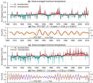
Figure 5a and c present the interannual variability of maxi-mum and minimaxi-mum temperature, respectively. Table 2 shows that Tmx exhibit frequencies between 2.4 and 3.5 years and of roughly 9 years while Tmn presents cycles between 3 and 6.5 years within the higher interannual band. The interannual modes strongly influence maximum temperature, explaining almost 60 % of its variability (see Table 2 and the IA re-construction signal, the grey line in Fig. 5a). Interestingly, Fig. 5b shows that the nearly 9-year cycle in Tmx correlates well (r=0.54; significant at the 99.8 % confidence level) with the main mode of the first global SST pattern (Fig. 2a), with signals over the Southern Atlantic, Indian and Pacific oceans. The interannual modes exhibit a weak effect on the minimum temperature (Fig. 5c) as they account for just 30 % of Tmn’s variability. Yet Fig. 5d shows that the minimum temperature is related to the ENSO mode with a periodicity close to 3 years, with warmer Tmn during El Niño years and cooler Tmn during La Niña events. These results are consis-tent with Müller et al. (2000) and Rusticucci et al. (2017), who reported that El Niño events intensify warm spells and reduce the number of climatological freezing days while La Niña events increase cold events.

4.2 Trends and decadal-to-multidecadal oscillations

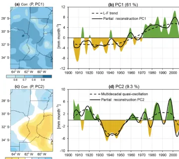
Figure 6a and b show the leading pattern of decadal-to-multidecadal precipitation variability. This pattern presents correlation values mostly larger than 0.7 and maximum val-ues towards the central-western portion of NEA. A notice-able nonlinear trend in the PC1 explains 60 % of its variance. The PC1 nonlinear trend shows two distinct periods of the precipitation: a dry one before 1970 and a wet one between 1970 and 2005. The wetting trend has stabilized and reversed starting in the 2000s (in agreement with Seager et al., 2010; Lovino et al., 2014; Saurral et al., 2017). The PC1 also ex-hibits interdecadal cycles of about 15–20 years (see Table 2). The second leading pattern of precipitation (Fig. 6c and d) displays negative correlations on the central-eastern portion of the domain and mostly weak positive correlations to the north and southwest. The PC2 has a near-decadal cycle and a multidecadal oscillation (Table 2) that explain 25 and 58 % of the PC2 variance respectively. As reported by Seager et al. (2010), Fig. 6b and d show that there was a multiyear period of droughts in the 1930s and 1940s coincident with negative anomalies in the low-frequency trend of PC1 and a dry episode of the multidecadal oscillation of PC2. This mul-tiyear drought was called the “Pampas Dust Bowl” (Viglizzo and Frank, 2006) and was caused by a hemispherical sym-metric pattern of precipitation anomalies with drought in both North and South America (Seager et al., 2010).

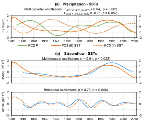
Figure 7a shows that the multidecadal oscillation of pre-cipitation (green line) has positive correlations with the PC2 (lf) SST (Interdecadal Pacific Oscillation, Sect. 3), and neg-ative correlation with the PC3 (lf) SST (Atlantic Multi-decadal Oscillation, Sect. 3). Thus, consistent with Seager et

al. (2010), Mo and Berbery (2011) and Barreiro et al. (2014), warm phases of the Interdecadal Pacific Oscillation and cold phases of the Atlantic Multidecadal Oscillation favor long-term wet anomalies in decadal timescales over NEA. It could be the case of the wet period from the 1970s to 2000s in gional precipitation as seen in Fig. 7a. Conversely, the re-versal in the wetting period since the mid-2000s can be ex-plained as a transition to a cold phase of the Pacific Ocean and a warm period of the Atlantic Ocean.

The low-frequency variability of the Paraná River stream-flow exhibits a nearly bidecadal and a multidecadal oscilla-tion that represent 20 and 60 % of the total variance respec-tively (Table 2). First, in agreement with Labat et al. (2005), Antico et al. (2014) and Antico et al. (2016), the top panel of Fig. 7b shows that the multidecadal oscillation of streamflow strongly correlates (r∼0.91, significant at the 98 % confi-dence level) with the low-frequency oscillation of the global SST (lf) PC2 related to the interdecadal Pacific variability. Thus, the warmest phase of the Interdecadal Pacific Oscilla-tion favored the extraordinary floods between 1980 and 2000 (see dots in Fig. 4a). Second, the bottom panel of Fig. 7b shows that the nearly bidecadal mode of streamflow corre-lates (r∼0.73; significant at the 95 % confidence level) with a similar mode in PC3 (lf) SST corresponding mainly to the North and South Atlantic (Fig. 2k). Thus, our results sug-gest that North and South Atlantic SSTs influence the Paraná River streamflow with bidecadal periodicities. In addition, Robertson and Mechoso (2000) and Antico et al. (2014) re-ported that the South Atlantic Convergence Zone also drives the Paraná River flow with 18-year periodicities.

Maximum and minimum near-surface temperatures also present a nearly bidecadal oscillation and a nonlinear trend (Table 2). The maximum temperature mostly varies with a bidecadal frequency (Fig. 5a) that induced larger values around the 1940s, 1960s and 2000s. The minimum tempera-ture is mostly dominated by a nonlinear trend (Fig. 5c) that favored a notable increase since the 1970s.

5 Sectoral impacts of hydroclimatic variability

-1 -0.5 0 0.5 1 -1 -0.5 0 0.5 1

1900 1910 1920 1930 1940 1950 1960 1970 1980 1990 2000 2010

S S T [º C ] T m x [º C ]

(b) Tmx - PC1 SST (T ~ 9 years; r = 0.54; p = 0.0021)

PC1 SST Tmx

1900 1910 1920 1930 1940 1950 1960 1970 1980 1990 2000 2010

-1.5 -0.5 0.5 1.5 2.5 18 m fi lte re d Tm x [º C ]

(a) Areal-averaged maximum temperature IA econstruction

LF econstruction

1900 1910 1920 1930 1940 1950 1960 1970 1980 1990 2000 2010

-1.5 -0.5 0.5 1.5 18 m fi lte re d Tm n [º C ]

(c) Areal-averaged minimum temperature IA econstruction

LF econstruction

-1 -0.5 0 0.5 1 -1 -0.5 0 0.5 1

1900 1910 1920 1930 1940 1950 1960 1970 1980 1990 2000 2010

S S T [ ºC ] T m n [º C ]

(d) Tmn - ENSO (T ~ 3.5 years; r = 0.35; p = 0.0824)

PC2 SST Tmn

r r

r r

Figure 5.Panels(a)and(c)present the 18 m low-pass-filtered monthly time series of areal-averaged daily maximum and minimum temper-ature anomalies (in shades) and their partial reconstructions (in lines) using all interannual and low-frequency variability modes described in Table 2. Panels(b)and(d)depict the temporal evolution of the dominant modes of regional temperature and the first two leading patterns of global SST variability.T denotes the dominant period of the leading modes, andrindicates the Pearson correlation coefficients between time series. Significance levels (p values) forr are estimated by combining 2000 Monte Carlo iterations considering autocorrelation by resampling in the frequency domain (Macias-Fauria et al., 2012).

5.1 Water resources

Water resources in northeastern Argentina are highly sensi-tive to hydroclimate variability and its extremes. Intense pre-cipitation events of shorter duration (days to weeks) origi-nated in mesoscale, and convective systems are common in NEA (Rasmussen et al., 2016). These events produce sud-den localized floods in plain areas that affect water resources management systems, i.e., cause severe complications in ur-ban and rural drainage systems (Bertoni et al., 2004). Persis-tent events (from seasons to years) affect water supply man-agement since groundwater, streamflow and reservoir storage reflect the longer-term precipitation anomalies (Latrubesse and Brea, 2011; Penalba and Rivera, 2016). These events, as discussed above, are mainly driven by extreme ENSO condi-tions that induce floods or droughts (row 1 of Table 3).

For instance, during the 2008–2009 and 2012 droughts the Salto Grande hydropower plant on the Uruguay River gener-ated only 10 % of its energy capacity, impacting on the

en-ergetic security of Uruguay and Argentina (El Día, 2012). These droughts affected navigability of the Paraná River, leading to complications to export grains and transport fuel (La Nación, 2009). The very low levels of the Paraná and Uruguay rivers hindered water extraction for supply, leading to shortages of drinking water and pollution problems (La Nación, 2009).

Our results show that northeastern Argentina suffered se-vere droughts that were more frequent before 1960, i.e., during the early 20th century (row 2 on Table 3). Dur-ing those years, the droughts severely affected regional economies with similar impacts to those discussed above but exacerbated by the scarce technological development at that time (Tasso, 2011).

ground-Figure 6.First two leading patterns of decadal-to-multidecadal precipitation variability characterized by the 120 m low-pass-filtered monthly mean precipitation anomalies. Panels(a)and(c)show the spatial distribution of the correlation between PCs (inbandd) and each precip-itation time series at a single grid point. Percentages of explained variance are given in brackets. Black lines depict the leading modes of variability (dashed) and the partial reconstruction of each PC using all modes described in Table 2 (continuous).

Table 3.Impacts of hydroclimate variability and its extremes in water resources. The first column shows the main timescale of variability affecting the study sector.

Timescale Key impacts in water resources Key references

Interannual Flooding mostly during El Niño years and droughts generally associated with La Niña events affect water management. Difficulties in water supply, hydroelectric power generation and river navigability.

Grimm et al. (2000) Grimm and Tedeschi (2009) Garreaud et al. (2009) Latrubesse and Brea (2011) Barros et al. (2015) Penalba and Rivera (2016)

Interannual to multidecadal Severe hydrological droughts, mainly in 1901– 1960.

Viglizzo and Frank (2006) Tasso et al. (2011) Lovino et al. (2014)

Decadal to multidecadal Increased precipitation caused increased flows. Frequent regional flooding between 1970 and 2005. Increased groundwater levels favored sur-face runoff. Extraordinary fluvial floods.

Venencio and García (2011) Latrubesse and Brea (2011) Cavalcanti (2012)

Figure 7.Time series of the dominant modes of regional hydrocli-mates variables and the leading patterns of global SSTs at decadal-to-multidecadal timescales. The description of the modes is given in Tables 1 and 2:(a)Multidecadal oscillations in PC2 SST, PC3 SST and PC2 P.(b)Multidecadal oscillations in streamflow and PC2 (top panel); bidecadal oscillation in streamflow and PC3 SSTs (bottom panel). The termrdenotes the Pearson correlation coefficient be-tween series. Significance levels (pvalues) forr are estimated by combining 2000 Monte Carlo iterations considering autocorrelation by resampling in the frequency domain (Macias-Fauria et al., 2012).

water table levels and favored increased surface runoff (e.g., Venencio and García, 2011; Latrubesse and Brea, 2011). All these changes combined with the significant hydrological variability on interannual timescales favored extraordinary floods in the main rivers in recent decades.

In 1983 and 1998, the extraordinary floods of the Paraná and Uruguay rivers forced the evacuation of hundreds of thousands of people and an estimated cost of over a billion dollars (Barros et al., 2015). During those years, the Paraná River floods affected approximately 40 000 km2for 8 months (Fritschy, 2010; Barros et al., 2015). Moreover, the Salado river – a tributary of the Paraná river – experienced its most catastrophic flood in 2003, causing economic losses of ap-proximately USD 1 billion and dozens of dead in the city of Santa Fe (ECLAC, 2003).

In the coming decades, it is expected that flooding in the Paraná River occurs frequently due to the influence of inter-annual variability. As noted in Sect. 4.2, the “positive” phase of the multidecadal hydrological variability that exacerbated the magnitude of floods during the 1980–2005 period was weakened in the last decade and could even reverse in the coming years. Our results suggest that the change of phase in multidecadal streamflow variability was induced by a rever-sal in the precipitation-wetting trend and in the multidecadal modes of streamflow. Seager et al. (2010) argued that the

re-versal of the precipitation trend is influenced by a shift to-ward a positive phase of the Atlantic Multidecadal Oscilla-tion (Ting et al., 2009), which may drive a precipitaOscilla-tion de-crease in the coming years. Thus, if these conditions remain, the influence of multidecadal variability could attenuate the magnitudes and devastating impacts of the floods compared to those that occurred during the 1980–2005 period.

5.2 Agriculture

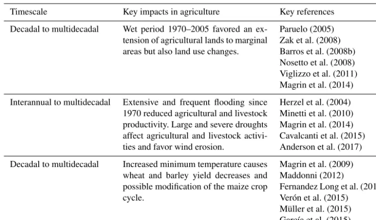
Agricultural activities were favored by the long-term wet pe-riod since 1970, improved technology and increased planted area: a significant increase in annual crops of around 60 % occurred in the whole region (Viglizzo et al., 2011). Wetter conditions also led to increases in crop yields (maize and soy-bean yields increased 9 and 58 % respectively; Magrin et al., 2007). The wet period since 1970 as well as economic, so-cial and technological drivers contributed to the expansion of agriculture over regions previously relegated, like the Chaco dry forest, toward the northwest of the study region (Paruelo, 2005). It leads to a strong process of land use changes: about 80 % of the natural forest has been converted to pastures, scrub or cropland (Zak et al., 2008; Viglizzo et al., 2011). According to Nosetto et al. (2008) and Magrin et al. (2014) those land use changes have disrupted natural water and bio-geochemical cycles, affecting surface runoff and salinizing the soil.

The combination of interannual and multidecadal hydro-logical variability led to extreme events (floods and droughts) that affected agricultural and livestock productivity (row 2 of Table 4). According to Magrin et al. (2014), river floods and extensive pluvial flooding, more frequent after 1970, af-fected riverine and rural areas causing losses or damages in pastures and crops and forcing displacement of cattle. For instance, the Paraná flood in 1998 affected 3.5 million pro-ductive hectares and caused losses of USD 750 million in the agricultural sector of Argentina (Herzel et al., 2004). The ex-tensive pluvial floods of 2016 affected 6 million productive hectares in the core crop region of Argentina, causing losses of USD 2750 million including crop damages, animal mor-tality, pasture and inputs, and the destruction of dairy farm equipment (La Nación, 2016).

Table 4.Impacts of hydroclimate variability and its extremes in agriculture. The first column shows the main timescale of variability affecting the study sector.

Timescale Key impacts in agriculture Key references

Decadal to multidecadal Wet period 1970–2005 favored an ex-tension of agricultural lands to marginal areas but also land use changes.

Paruelo (2005) Zak et al. (2008) Barros et al. (2008b) Nosetto et al. (2008) Viglizzo et al. (2011) Magrin et al. (2014)

Interannual to multidecadal Extensive and frequent flooding since 1970 reduced agricultural and livestock productivity. Large and severe droughts affect agricultural and livestock activi-ties and favor wind erosion.

Herzel et al. (2004) Minetti et al. (2010) Magrin et al. (2014) Cavalcanti et al. (2015) Anderson et al. (2017)

Decadal to multidecadal Increased minimum temperature causes wheat and barley yield decreases and possible modification of the maize crop cycle.

Magrin et al. (2009) Maddonni (2012)

Fernandez Long et al. (2013) Verón et al. (2015)

Müller et al. (2015) García et al. (2015)

2008 reduced crop yields by 40 % and caused the mortality of 700 000 cattle (La Nación, 2008).

The variability and changes in temperature also affect the agricultural and livestock sector (row 3 of Table 4). The in-crease in minimum temperature results in inin-creased wheat and barley respiration rates and shorter grain-filling periods, diminishing their yields (Magrin et al., 2009; Verón et al., 2015). According to García et al. (2015), wheat and barley yields were reduced by 7 % under increased minimum tem-peratures without considering technological improvements. The life cycle of maize has been affected by fewer frost events that allow early planting dates (Maddonni, 2012).

5.3 Human settlements

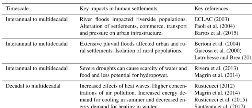
Frequent pluvial and river floods affected urban and rural populations in the Lower Paraná basin (rows 1 and 2 of Ta-ble 5). River floods affect mostly vulneraTa-ble social sectors such as unplanned urban settlements, usually located in river floodplain areas, while pluvial floods affect established rural and urban populations spread over large areas of the Pampas. There are many reported cases of severe damage to cities due to river floods. For instance, the Paraná River flood in 1982–1983 inundated 70 % of the city of Resistencia (located on the opposite margin of the river from the city of Corri-entes) and forced the evacuation of 91 500 people (Herzel et al., 2004). The sewer system, urban drainage, and the power system collapsed and the communication lines disrupted, re-sulting in economic losses of USD 150 million (Caputo et al., 1985). According to ECLAC (2003), the Salado River flood in the city of Santa Fe in 2003 forced the evacuation of 120 000 people and affected 20 000 houses. This disaster

re-sulted in severe damage to urban infrastructure estimated at USD 450 million including drinking water and sanitation, en-ergy, and transportation and telecommunications networks. Moreover, the extraordinary river floods also affected rural settlements. For instance, the Paraná River flood of 1998 af-fected 53 000 families of small farmers, rural workers and indigenous communities (Herzel et al., 2004).

Pluvial floods have frequently affected small settlements in the NEA, but have also led to major disasters in densely populated cities. In 2013, an unprecedented intense rainfall that reached 400 mm in less than 12 h flooded the city of La Plata, the capital city of the province of Buenos Aires. In the urban area, 3500 hectares were flooded, more than 80 people died and more than 190 000 people were affected and sub-stantial material damage was caused (UNLP, 2013). The city of Santa Fe suffered a pluvial flood in 2007 that affected a great part of the urban area, causing three deaths and forcing the evacuation of 26 000 people (La Nación, 2007).

consump-Table 5.Impacts of hydroclimate variability and its extremes in human settlements. The first column shows the main timescale of variability affecting the study sector.

Timescale Key impacts in human settlements Key references

Interannual to multidecadal River floods impacted riverside populations. Alteration of settlements, commerce, transport and pressure on urban infrastructure.

ECLAC (2003) Paoli et al. (2004) Barros et al. (2015)

Interannual to multidecadal Extensive pluvial floods affected urban and ru-ral settlements. Isolation of ruru-ral populations.

Bertoni et al. (2004) Giacosa et al. (2000) Latrubesse and Brea (2011)

Interannual to multidecadal Severe droughts can cause scarcity of water and food and less potential for hydropower.

Rivera et al. (2013) Magrin et al. (2014)

Decadal to multidecadal Increased effects of heat waves. Higher concen-trations of air pollution. Increased energy de-mand for cooling in summer and decreased en-ergy demand for heating in winter.

Rusticucci (2012) Magrin et al. (2014) Rusticucci et al. (2015) Santágata et al. (2017)

tion for heating during winter and increases for cooling dur-ing summers (Santágata et al., 2017). For instance, Argentina suffered an intense heat wave that killed seven people in De-cember 2013 (BBC News, 2013). The intense heat was exac-erbated by power cuts and water shortages, leading to hun-dreds of cases of heatstroke in Buenos Aires (Independent, 2013).

6 Final remarks

Hydroclimate variability (here described by precipitation, streamflow and near-surface temperature) impacts water re-sources, agriculture and human settlements in northeastern Argentina, exacerbating social, political, economic and en-vironmental risks already existing in the region. This study (a) investigated the regional hydroclimate variability on interannual-to-multidecadal timescales, (b) reviewed and ad-vanced the understanding of its links with global SSTs forc-ing, and (c) discussed the impacts of hydroclimate variability and its extremes on the main productive and socioeconomic regional sectors.

The region is affected by hydroclimate variability modes in different timescales, from interannual to multidecadal, and likely by different trends. Our results suggest that short-period cycles of the ENSO-related interannual precipitation variability over NEA (a) favored extreme events after 2000, even during moderate extreme phases of the ENSO (period-icities of 2–4 years), and (b) contributed to the Low Paraná river streamflow with periodicities of nearly 2 years. Al-though precipitation rates over NEA account for a small per-centage of the total Paraná River flow, the latter finding can provide valuable information to improve flood early warn-ing systems in periods of low flow contribution in the middle and upper reaches of the river. Regarding temperature, min-imum temperature relates to ENSO with a main frequency

close to 3 years. Maximum temperature time series correlate well with SSTs variability over the Southern Atlantic, Indian and Pacific oceans, with a 9-year frequency. On decadal-to-multidecadal timescales, in addition to the known incidence of the Interdecadal Pacific Oscillation and the Atlantic Multi-decadal Oscillation that favor long-term anomalies over NEA (Seager et al., 2010; Barreiro et al., 2014), this study reports that the Paraná River streamflow is influenced by North and South Atlantic SSTs with bidecadal periodicities.

Interannual hydrological variability induced frequent floods and droughts that are mainly related to extreme ENSO conditions, often combined with SST forcing in the North Tropical Atlantic Ocean and the South Atlantic Convergence Zone. These extreme events altered the management of sur-face and groundwater resources. Frequent floods affected agricultural and livestock productivity in riverine and rural areas of the Pampas, causing damages to pastures and crops and forcing displacement of cattle. Human settlements were also affected, including impacts on trade, transportation, and infrastructure of urban and rural populations. Conversely, agricultural droughts disrupted seeding or critical periods of crops and hydrological droughts impacted water supply for cattle while favoring soil erosion. The most severe hydrolog-ical droughts directly affected the population, causing water and food scarcity and reducing the potential for hydropower generation.

low-frequency timescales affected productive sectors and ur-ban settlements. Increases in minimum temperature reduced wheat yields and altered maize life cycles. Changes in max-imum and minmax-imum temperatures exacerbated the effects of urban heat islands and affected energy demand in several cities of the region.

The combination of interannual and multidecadal hydro-climatic variability intensified extreme events in the past, leading to the most severe droughts in the early 20th century and largest floods after 1970. Since the mid-2000s, northeast-ern Argentina has been showing signs of a reversal in the wet-ting period on multidecadal timescales. If these conditions continue into the coming decades, more severe droughts and weaker floods might be expected. Considering the relevance of the multidecadal variability in the formation of extreme events, this information should be monitored and incorpo-rated into regional decision systems to improve planning by water managers and agricultural stakeholders.

Data availability. GPCC v7 and CRU TS 3.25 data sets are

available at https://doi.org/10.5676/DWD_GPCC/FD_M_V7_050 (Schneider et al., 2015) and

https://doi.org/10.5285/c311c7948e8a47b299f8f9c7ae6cb9af (Uni-versity of East Anglia Climatic Research Unit, 2017). The Paraná River streamflow data were provided by the Integrated Hydrological Data Base of the National Water Information System of Argentina (available at http://bdhi.hidricosargentina.gob.ar).

Competing interests. The authors declare that they have no conflict

of interest.

Acknowledgements. This research was carried out with the support

of Project CRN3035 of the Inter-American Institute for Global Change Research (IAI), which is supported by the US National Science Foundation. UNL Project C.A.I.+D. 2011 35/180 are also acknowledged. We greatly appreciate the support of Ernesto H. Berbery in the preparation of this paper. We are grateful to the anonymous reviewers whose constructive comments and recommendations helped to improve the paper.

Edited by: Luis Samaniego

Reviewed by: two anonymous referees

References

Anderson, W., Seager, R., Baethgen, W., and Cane, M.: Life cycles of agriculturally relevant ENSO teleconnections in North and South America, Int. J. Climatol., 37, 3297–3318, https://doi.org/10.1002/joc.4916, 2017.

Andrade, M. I. and Scarpati, O. E.: Recent changes in flood risk in the Gran La Plata, Buenos Aires Province, Argentina: causes and management strategy, GeoJournal, 70, 245–250, https://doi.org/10.1007/s10708-008-9137-9, 2007.

Andreoli, R. V. and Kayano, M. T.: ENSO-related rainfall anoma-lies in South America and associated circulation features during warm and cold Pacific Decadal Oscillation regimes, Int. J. Cli-matol., 25, 2017–2030, https://doi.org/10.1002/joc.1222, 2005. Antico, A., Schlotthauer, G., and Torres, M. E.:

Analy-sis of hydroclimatic variability and trends using a novel empirical mode decomposition: Application to the Paraná River Basin, J. Geophys. Res.-Atmos., 119, 1218–1233, https://doi.org/10.1002/2013JD020420, 2014.

Antico, A., Torres, M. E., and Diaz, H.: Contributions of different time scales to extreme Paraná floods, Clim. Dynam., 46, 3785– 3792, https://doi.org/10.1007/s00382-015-2804-x, 2016. Baethgen, W. E. and Goddard, L.: Latin American Perspectives

on Adaptation of Agricultural Systems to Climate Variability and Change, in: Handbook of Climate Change and Agroecosys-tems: Global and Regional Aspects and Implications, edited by: Hillel, D. and Rosenzweig, C., Imperial College Press, 57–72, https://doi.org/10.1142/9781848169845_0004, 2013.

Barreiro, M., Diaz, N., and Renom, M.: Role of the global oceans and land–atmosphere interaction on summertime interdecadal variability over northern Argentina, Clim. Dynam., 42, 1733– 1753, https://doi.org/10.1007/s00382-014-2088-6, 2014. Barros, V., Menendez, A., Natenzon, C., Kotot, R., Codignotto, J.,

Re, M., Bronstein, P., Camillon, I., Luduena, S., Rios, D., and Gonzalez, S. G.: Storm surges, rising seas and flood risks in metropolitan Buenos Aires. Climate Change and Vulnerability, edited by: Leary, N., Conde, C., Kulkarni, J., Nyong, A., and Pulhin, J., Earthscan, 117–133, 2008a.

Barros, V., Doyle, M., and Camilloni, I.: Precipitation trends in southeastern South America: Relationship with ENSO phases and with low-level circulation, Theor. Appl. Climatol., 93, 19– 33, https://doi.org/10.1007/s00704-007-0329-x, 2008b. Barros, V. R., Boninsegna, J. A., Camilloni, I. A., Chidiak, M.,

Magrín, G. O., and Rusticucci, M.: Climate change in Ar-gentina: trends, projections, impacts and adaptation, WIREs Clim. Change, 6, 151–169, https://doi.org/10.1002/wcc.316, 2015.

Barrucand, M., Rusticucci, M., and Vargas, W.: Tempera-ture extremes in the south of South America in rela-tion to Atlantic Ocean surface temperature and Southern Hemisphere circulation, J. Geophys. Res., 113, D20111, https://doi.org/10.1029/2007JD009026, 2008.

BBC News: Heatwave kills seven in Argentina, available at: http:// www.bbc.com/news/world-latin-america-25564633 (last access: 7 August 2017), 2013.

Berbery, E. H. and Barros, V.: The hydrologic cy-cle of the La Plata basin in South America, J. Hy-drometeor., 3, 630–645, https://doi.org/10.1175/1525-7541(2002)003<0630:THCOTL>2.0.CO;2, 2002.

Bertoni, J. C.: Urbanization and urban drainage in Argentina, in: urban floods in Argentina, edited by: Bertoni, J. C., Córdoba, chap. 3, Argentina, 43–74, 2004 (in Spanish).

Bidegain, M.: Severe drought in central Argentina and Uruguay, in: State of the Climate in 2008, B. Am. Meteorol. Soc., 90, p. S138, 2009.

Camilloni, I. and Barros, V.: Extreme discharge events in Paraná River and their climate forcing, J. Hydrol., 278, 94–106, https://doi.org/10.1016/S0022-1694(03)00133-1, 2003. Caputo, G., Hardoy, J., and Herzer, H.: La inundación en el Gran

Resistencia. Evaluación de las respuestas frente a la emergen-cia, in: Inundaciones y Sociedad en el Gran Resistencia Chaco l982–83, Ediciones Boletín de Medio Ambiente y Urbanización de la Comisión de Desarrollo Urbano y Regional. Buenos Aires, CLACSO/GEL, 1985 (in Spanish).

Carril, A. F., Cavalcanti, I. F. A., Menéndez, C. G., Sörensson, A., López-Franca., N., Rivera, J., Robledo, F., Zaninelli, P., Am-brizzi, T., Penalba, O., da Rocha, R., Sánchez, E., Bettolli, M., Pessacg, N., Renom, M., Ruscica, R., Solman, S., Tencer, B., Grimm, A., Rusticucci, M., Cherchi, A., Tedeschi, R., and Zam-boni, L.: Extreme events in the La Plata basin: a retrospective analysis of what we have learned during CLARIS-LPB project, Clim. Res., 68, 95–116, https://doi.org/10.3354/cr01374, 2016. Carter, L. M., Cohen, S. J., Grimm, N. B., and Hatfield, J. L.:

Weather and Climate Extremes in a Changing Climate, Regions of Focus: North America, Hawaii, Caribbean and U.S. Pacific Islands, Synthesis and Assessment Product 3.3, Report by the US Climate Change Science Program and the Subcommittee on Global Change, Washington, DC, 162 pp., 2008.

Cavalcanti, I. F. A.: Large scale and synoptic features associated with extreme precipitation over South America: a review and case studies for the first decade of the 21st century, Atmos. Res., 118, 27–40, https://doi.org/10.1016/j.atmosres.2012.06.012, 2012.

Cavalcanti, I. F. A., Carril, A. F., Penalba, O. C., Grimm, A. M., Menéndez, C. G., Sanchez, E., Chechi, A., Sörens-son, A., Robledo, F., Rivera, J., Pántano, V., Betolli, L. M., Zaninelli, P., Zamboni, L., Tedeschi, R. G., Dominguez, M., Ruscica, R., and Flach, R.: Precipitation extremes over La Plata Basin – review and new results from observa-tions and climate simulaobserva-tions, J. Hydrol., 523, 211–230, https://doi.org/10.1016/j.jhydrol.2015.01.028, 2015.

Coronel, G. and Menéndez, G.: Physiography and hydrology, in: Climatic Change in the La Plata Basin, edited by: Barros, V., Clarke, R., Diaz, P., National Scientific and Technical Research Council (CONICET), Argentina, 44–59, 2006.

Deser, C., Alexander, M. A., Xie, S.-P., and Phillips A. S.: Sea Sur-face Temperature Variability: Patterns and Mechanisms, Annu. Rev. Mar. Sci., 2, 115–143, https://doi.org/10.1146/annurev-marine-120408-151453, 2010.

Duchon, C. E.: Lanczos filtering in one and two dimensions, J. Appl. Meteorol., 18, 1016–1022, https://doi.org/10.1175/1520-0450(1979)018<1016:LFIOAT>2.0.CO;2, 1979.

Duchon, C. and Hare, R.: Filtering Data, in: Time Series Analysis in Meteorology and Climatology: An Introduction, chap. 3, John Wiley & Sons, New York, USA, 143–182, 2012.

ECLAC (United Nations Economic Commission for Latin America and the Caribbean): Evaluación del impacto de las inundaciones y el desbordamiento del Río Salado en la provincia de Santa Fe, República Argentina, 2003, available at: http://www.cepal.org/es/publicaciones/28461-evaluacion- impacto-inundaciones-desbordamiento-rio-salado-la-provincia-santa-fe (last access: 5 August 2017), 2003 (in Spanish). El Día: La represa de Salto Grande genera un 10% de

energía debido a la escasez de lluvias, available at:

http://www.eldiaonline.com/la-represa-de-salto-grande-genera-un-10-de-energia-debido-a- la-escasez-de-lluvias/ (last access: 2 August 2017), 2012 (in Spanish).

El Economista: Las últimas dos sequías costaron Us$ 8.675 millones, available at: http://www.eleconomista.com.ar/ 2016-10-las-ultimas-dos-sequias-costaron-us-8-675-millones/ (last access: 7 August 2017), 2016 (in Spanish).

Enfield, D., Mestas-Nuñez, A., and Trimble, P.: The Atlantic Mul-tidecadal Oscillation and its relation to rainfall and river flows in the continental U.S, Geophys. Res. Lett., 28, 2077–2080, https://doi.org/10.1029/2000GL012745, 2001.

Fernandez Long, M. E., Müller, G. V., Beltrán-Przekurat, A., and Scarpati, O.: Long- and short- term changes in temperature-based agroclimatic indices in argentina, Int. J. Climatol., 33, 1673– 1686, https://doi.org/10.1002/joc.3541, 2013.

Field, C. B., Barros, V. R., Mach, K. J., Mastrandrea, M. D., van Aalst, M., Adger, W. N., Arent, D. J., Barnett, J., Betts, R., Bilir, T. E., Birkmann, J., Carmin, J., Chadee, D. D., Challinor, A. J., Chatterjee, M., Cramer, W., Davidson, D. J., Estrada, Y. O., Gattuso, J.-P., Hijioka, Y., Hoegh-Guldberg, O., Huang, H. Q., Insarov, G. E., Jones, R. N., Kovats, R. S., Romero-Lankao, P., Larsen, J. N., Losada, I. J., Marengo, J. A., McLean, R. F., Mearns, L. O., Mechler, R., Morton, J. F., Niang, I., Oki, T., Olwoch, J. M., Opondo, M., Poloczanska, E. S., Pörtner, H.-O., Redsteer, M. H., Reisinger, A., Revi, A., Schmidt, D. N., Shaw, M. R., Solecki, W., Stone, D. A., Stone, J. M. R., Strzepek, K. M., Suarez, A. G., Tschakert, P., Valentini, R., Vicuña, S., Vil-lamizar, A., Vincent, K. E., Warren, R., White, L. L., Wilbanks, T. J., Wong, P. P., and Yohe, G. W.: Technical summary. in: Climate Change 2014: Impacts, Adaptation, and Vulnerability. Part A: Global and Sectoral Aspects. Contribution of Working Group II to the Fifth Assessment Report of the Intergovernmen-tal Panel on Climate Change, edited by: Field, C. B., Barros, V. R., Dokken, D. J., Mach, K. J., Mastrandrea, M. D., Bilir, T. E., Chatterjee, M., Ebi, K. L., Estrada, Y. O., Genova, R. C., Girma, B., Kissel, E. S., Levy, A. N., MacCracken, S., Mastrandrea, P. R., and White, L. L., Cambridge University Press, Cambridge, United Kingdom and New York, NY, USA, 35–94, 2014. Fritschy, B. A.: Impacto de las inundaciones

extraordinar-ias. Santa Fe, Argentina, Tercer Simposio Internacional de Investigación-SII, San Salvador de Jujuy, Jujuy, Ar-gentina, available at: http://www.siagua.org/sites/default/files/ documentos/documentos/inundaciones_extraordinarias.pdf (last access: 5 August 2017), 2010 (in Spanish).

García, N. O. and Mechoso, C. R.: Variability in the discharge of South American rivers and in Climate, Hydrolog. Sci. J., 50, 459–478, https://doi.org/10.1623/hysj.50.3.459.65030, 2005. García, G. A., Dreccer, M. F., Miralles, D. J., and Serrago, R. A.:

High night temperatures during grain number determination re-duce wheat and barley grain yield: a field study, Glob. Change Biol., 21, 4153–4164, https://doi.org/10.1111/gcb.13009, 2015. Garreaud, R. D., Vuille, M., Compagnucci, R., and Marengo, J.:

Present-day South American climate, Paleogeogr. Paleocl., 281, 180–195, https://doi.org/10.1016/j.palaeo.2007.10.032, 2009. Ghil, M., Allen, M., Dettinger, M. D., Ide, K., Kondrashov,

Giacosa, R. H.: Knowing the hydrological regime, in: The Parana River in its middle section: a contribution to knowledge and en-gineering practices in a large lowland river, edited by: Paoli, C. and Schreider, M., UNL publications, 69–103, 2000 (in Spanish). Grimm, A. M., Barros, V. R., and Doyle, M. E.: Climate variabil-ity in southern South America associated with El Niño and La Niña events, J. Climate, 13, 35–58, https://doi.org/10.1175/1520-0442(2000)013<0035:CVISSA>2.0.CO;2, 2000.

Grimm, A. M. and Tedeschi, R. G.: ENSO and Extreme Rainfall Events in South America, J. Climate, 22, 1589– 1609, https://doi.org/10.1175/2008JCLI2429.1, 2009.

Grimm, A. M. and Saboia, J. P. J.: Interdecadal variability of the South American precipitation in the monsoon season, J. Climate, 28, 755–775, https://doi.org/10.1175/JCLI-D-14-00046.1, 2015. Grimm, A. M., Laureanti, N. C., Rodakoviski, R. B., and Gama, C. B.: Interdecadal variability and extreme precipitation events in South America during the monsoon season, Clim. Res., 68, 277–294, https://doi.org/10.3354/cr01375, 2016.

Harris, I., Jones, P. D., Osborn, T. J., and Lister, D. H.: Up-dated high-resolution grids of monthly climatic observations – the CRU TS3.10 Dataset, Int. J. Climatol., 34, 623–642, https://doi.org/10.1002/joc.3711, 2014.

Haylock, M. R., Peterson, T. C., Alves, L. M., Ambrizzi, T., Anun-ciação, Y. M. T., Baez, J., Barros, V. R., Berlato, M. A., Bidegain, M., Coronel, G., Corradi, V., Garcia, V. J., Grimm, A. M., Karoly, D., Marengo, J. A., Marino, M. B., Moncunill, D. F., Nechet, D., Quintana, J., Rebello, E., Rusticucci, M., Santos, J. L., Trebejo, I., and Vincent, L. A.: Trends in total and extreme South Ameri-can rainfall in 1960–2000 and links with sea surface temperature, J. Climate, 19, 1490–1512, https://doi.org/10.1175/JCLI3695.1, 2006.

Henley, B. J., Gergis, J., Karoly, D. J., Power, S. B., Kennedy, J., and Folland, C. K.: A Tripole Index for the Inter-decadal Pacific Oscillation, Clim. Dynam., 45, 3077–3090, https://doi.org/10.1007/s00382-015-2525-1, 2015.

Hernandez, V., Moron, V., Riglos, F. F., and Muzi, E.: Con-fronting Farmers’ Perceptions of Climatic Vulnerability with Observed Relationships between Yields and Climate Vari-ability in Central Argentina, Weather Clim. Soc., 7, 39–59, https://doi.org/10.1175/WCAS-D-13-00062.1, 2015.

Herzel, H., Caputo, M. G., and Celis, A.: Capítulo III: Análi-sis regional: cuenca del río Paraná, in: Gestión de riesgos de desastre ENSO en América Latina, Informe Final IAI, Centro de estudios sociales y ambientales, available at: http://www.cambioglobal.org/enso/informes/anho4/Argentina/ Cap3CUENCADELPARANA.pdf (last access: 7 August 2017), 2004 (in Spanish).

Huang, H., Seager, R., and Kushnir, Y.: The 1976/77 transition in precipitation over the Americas and the influence of tropical SST, Clim. Dynam., 24, 721–740, https://doi.org/10.1007/s00382-005-0015-6, 2005.

Huang, B., Banzon, V. F., Freeman, E., Lawrimore, J., Liu, W., Peterson, T. C., Smith, T. M., Thorne, P. W., Woodruff, S. D., and Zhang, H.: Extended Reconstructed Sea Surface Tempera-ture Version 4 (ERSST.v4). Part I: Upgrades and Intercompar-isons, J. Climate, 28, 911–930, https://doi.org/10.1175/JCLI-D-14-00006.1, 2015.

Independent: Seven people die in the worst heat wave ever recorded in Argentina, available at:

http://www.independent.co.uk/news/world/americas/seven- people-die-in-the-worst-heat-wave-ever-recorded-in-argentina-9032202.html (last access: 7 August 2017), 2013.

Infocampo: Una catástrofe climática se extiende por más de la mitad del área agrícola argentina, available at: http://www.infocampo.com.ar/crea-una-catastrofe-climatica-se-extiende-por-mas-de-la-mitad-del -area-agricola-argentina/ (last access: 7 August 2017), 2009.

Jacques-Coper, M. and Garreaud, R. D.: Characterization of the 1970s climate shift in South America, Int. J. Climatol., 35, 2164– 2179, https://doi.org/10.1002/joc.4120, 2015.

Kosatsky, T.: The 2003 European heatwaves, Euro Surveillance, 10, 148–149, https://doi.org/10.2807/esm.10.07.00552-en, 2005. Krepper, C. M. and García, N. O.: Spatial and temporal structure of

trends and interannual variability of precipitation over La Plata Basin, Quartern. Int., 114, 11–21, https://doi.org/10.1016/S1040-6182(03)00038-7, 2004.

Krepper, C. M., García, N. O., and Jones, P. D.: Low-frequency response of the upper Paraná basin, Int. J. Climatol., 28, 351– 360, https://doi.org/10.1002/joc.1535, 2008.

Krepper, C. M. and Zucarelli, G. V.: Climatology of water excesses and shortages in the La Plata Basin, Theor. Appl. Climatol., 102, 13–27, https://doi.org/10.1007/s00704-009-0234-6, 2010. Labat, D., Ronchail, J., and Guyot, J. L.: Recent advances in

wavelet analyses: Part 2-Amazon, Parana, Orinoco and Congo discharges time scale variability, J. Hydrol., 314, 289–311, https://doi.org/10.1016/j.jhydrol.2005.04.004, 2005.

La Nación: Lluvias récord en Santa Fe: 3 muertos y 26.000 evacuados, available at: http://www.lanacion.com.ar/ 896183-lluvias-record-en-santa-fe-3-muertos-y-26000-evacuados (last access: 7 August 2017), 2007 (in Spanish).

La Nación: El campo padece la sequía más grave en dos décadas, available at: http://www.lanacion.com.ar/ 1044833-el-campo-padece-la-sequia-mas-grave-en-dos-decadas (last access: 7 August 2017), 2008 (in Spanish).

La Nación: Preocupa la histórica bajante en los ríos Uruguay y Paraná, available at: http://www.lanacion.com.ar/ 1130139-preocupa-la-historica-bajante-en-los-rios-uruguay-y-parana (last access: 2 August 2017), 2009 (in Spanish).

La Nación: Inundaciones: crecen las pérdidas productivas y económicas, available at: http://www.lanacion.com.ar/ 1893914-inundaciones-crecen-las-perdidas-productivas-y-economicas (last access: 7 August 2017), 2016 (in Spanish).

Latrubesse, E. and Brea, D.: Floods in Argentina, in: Natural Haz-ard and human-exacerbated disaster in Latin America, edited by: Latrubesse E., Elsevier, 333–349, 2011.

Liu, W., Huang, B., Thorne, P. W., Banzon, V. F., Zhang, H., Freeman, E., Lawrimore, J., Peterson, T. C., Smith, T. M., and Woodruff, S. D.: Extended Reconstructed Sea Surface Temperature Version 4 (ERSST.v4): Part II. Parametric and Structural Uncertainty Estimations, J. Climate, 28, 931–951, https://doi.org/10.1175/JCLI-D-14-00007.1, 2015.

Loikith, P. C., Detzer, J., Mechoso, C. R., Lee, H., and Barkhor-darian, A.: The influence of recurrent modes of climate vari-ability on the occurrence of monthly temperature extremes over South America, J. Geophys. Res.-Atmos., 122, 10297–10311, https://doi.org/10.1002/2017JD027561, 2017.