The sensitivity of modeled snow accumulation and melt to precipitation phase methods across a climatic gradient

https://doi.org/10.5194/hess-23-3765-2019 © Author(s) 2019. This work is distributed under the Creative Commons Attribution 4.0 License.

The sensitivity of modeled snow accumulation and melt to

precipitation phase methods across a climatic gradient

Keith S. Jennings1,2,3,4and Noah P. Molotch1,2,5

1_{Geography Department, University of Colorado Boulder, 260 UCB, Boulder, Colorado 80309, USA}

2_{Institute of Arctic and Alpine Research, University of Colorado Boulder, 450 UCB, Boulder, Colorado 80309, USA} 3_{Department of Geography, University of Nevada, Reno, 1664 N. Virginia Street, Reno, Nevada 89557, USA} 4_{Desert Research Institute, 2215 Raggio Parkway, Reno, Nevada 89512, USA}

5_{NASA Jet Propulsion Laboratory, 4800 Oak Grove Drive, Pasadena, California 91109, USA}

Correspondence:Keith S. Jennings ([email protected])

Received: 15 February 2019 – Discussion started: 5 March 2019

Revised: 16 July 2019 – Accepted: 10 August 2019 – Published: 18 September 2019

Abstract. A critical component of hydrologic modeling in cold and temperate regions is partitioning precipitation into snow and rain, yet little is known about how uncertainty in precipitation phase propagates into variability in simulated snow accumulation and melt. Given the wide variety of meth-ods for distinguishing between snow and rain, it is impera-tive to evaluate the sensitivity of snowpack model output to precipitation phase determination methods, especially con-sidering the potential of snow-to-rain shifts associated with climate warming to fundamentally change the hydrology of snow-dominated areas. To address these needs we quantified the sensitivity of simulated snow accumulation and melt to rain–snow partitioning methods at sites in the western United States using the SNOWPACK model without the canopy module activated. The methods in this study included dif-ferent permutations of air, wet bulb and dew point temper-ature thresholds, air tempertemper-ature ranges, and binary logistic regression models. Compared to observations of snow depth and snow water equivalent (SWE), the binary logistic regres-sion models produced the lowest mean biases, while high and low air temperature thresholds tended to overpredict and un-derpredict snow accumulation, respectively. Relative differ-ences between the minimum and maximum annual snowfall fractions predicted by the different methods sometimes ex-ceeded 100 % at elevations less than 2000 m in the Oregon Cascades and California’s Sierra Nevada. This led to ranges in annual peak SWE typically greater than 200 mm, exceed-ing 400 mm in certain years. At the warmer sites, ranges in snowmelt timing predicted by the different methods were

generally larger than 2 weeks, while ranges in snow cover du-ration approached 1 month and greater. Conversely, the three coldest sites in this work were relatively insensitive to the choice of a precipitation phase method, with average ranges in annual snowfall fraction, peak SWE, snowmelt timing, and snow cover duration of less than 18 %, 62 mm, 10 d, and 15 d, respectively. Average ranges in snowmelt rate were typically less than 4 mm d−1and exhibited a small relationship to sea-sonal climate. Overall, sites with a greater proportion of pre-cipitation falling at air temperatures between 0 and 4◦C ex-hibited the greatest sensitivity to method selection, suggest-ing that the identification and use of an optimal precipitation phase method is most important at the warmer fringes of the seasonal snow zone.

1 Introduction

uniform air temperature threshold or a range between two thresholds with a linear mix of liquid and solid precipitation in between. Recent work has called this simplistic treatment of precipitation phase into question (Feiccabrino et al., 2015; Harpold et al., 2017b) because of the pronounced spatial vari-ability in rain–snow partitioning (Jennings et al., 2018b; Ye et al., 2013). Complicating matters is the fact that precipita-tion phase is rarely observed in mountain regions on a con-tinuous basis over long timescales.

The use of a spatially uniform air temperature threshold is seemingly logical given the strong temperature dependence of precipitation phase. Observational work has shown that precipitation is primarily solid at temperatures at and below the freezing point (Auer, 1974; Avanzi et al., 2014; United States Army Corps of Engineers, 1956) and that the proba-bility of snowfall decreases following a sigmoidal curve as air temperature increases above 0◦_{C (Dai, 2008; Fassnacht}

et al., 2013; Kienzle, 2008). However, the point at which the sigmoidal curve crosses 50 % snow probability (i.e., the 50 % rain–snow air temperature threshold) has been shown to vary significantly across the Northern Hemisphere (Jen-nings et al., 2018b). Thus, a single air temperature threshold, or range, cannot accurately represent precipitation phase par-titioning across large spatial extents (Raleigh and Lundquist, 2012). Part of this variability can be ascribed to relative humidity, as recent work has shown that snowfall is more probable at a given air temperature in more arid conditions (Froidurot et al., 2014; Gjertsen and Ødegaard, 2005; Jen-nings et al., 2018b). Surface air pressure also affects phase partitioning, but to a lesser degree than air temperature and humidity, with snowfall being more common at higher air temperatures when surface pressure is lower (Ding et al., 2014; Jennings et al., 2018b; Rajagopal and Harpold, 2016). Given the secondary controls exerted by humidity and sur-face pressure on the probability of rain versus snow, precip-itation phase methods have been developed to leverage this information into more accurate rain and snow predictions. These methods include dew point temperature thresholds (Marks et al., 2013; Ye et al., 2013), wet and ice bulb tem-perature thresholds (Anderson, 1968; Harder and Pomeroy, 2013), and binary logistic regression equations that predict the probability of snow as a function of various meteorologi-cal quantities (Froidurot et al., 2014). In general, methods in-corporating humidity better predict precipitation phase than methods using air temperature alone relative to observations across the Northern Hemisphere (Jennings et al., 2018b), likely due to their better representation of the hydrometeor energy balance (Harder and Pomeroy, 2013; Harpold et al., 2017b). Furthermore, the spatial variability in phase parti-tioning is reduced when using humidity information in addi-tion to air temperature (Ye et al., 2013).

This wide variety of precipitation phase methods leads to variations in snowfall fraction – the percentage of annual pre-cipitation that falls as snow – approaching 30 % or greater when applied to station meteorological data and

reanaly-sis products (Harpold et al., 2017c; Jennings et al., 2018b; Raleigh et al., 2016). This previous work has shown that warmer sites are generally more sensitive to precipitation phase method selection in terms of annual snowfall frac-tion variability, though it is less certain how this variabil-ity translates into divergences in simulated snow accumu-lation and melt. To that end, Harder and Pomeroy (2014) showed that precipitation phase method selection can pro-duce ranges in annual peak snow water equivalent (SWE) and snow cover duration of 160 mm and 36 d, respectively. However, this work only examined relatively cold research basins in Canada and did not consider the warmer mid-latitude, maritime climates that have been shown to be most “at risk” of the effects of climate warming on snow accu-mulation (e.g., Nolin and Daly, 2006). Similarly, other re-searchers have found that higher air temperature thresholds generate greater annual peak SWE and increased snow accu-mulation during storm events at individual sites and basins (Fassnacht and Soulis, 2002; Mizukami et al., 2013; Wayand et al., 2017; Wen et al., 2013).

We are therefore left with the question of how the sensi-tivity of modeled snow accumulation and melt to precipita-tion phase method selecprecipita-tion varies across sites with differ-ent climatic characteristics. Considering that over 1 billion people worldwide rely on mountain snowpacks for water re-sources (Barnett et al., 2005; Mankin et al., 2015), it is essen-tial that models accurately represent precipitation phase par-titioning as well as snowpack water storage and snowmelt timing. Furthermore, snowpacks are highly reflective rela-tive to bare ground, meaning that simulated snow cover dura-tion has a significant effect on modeled land surface albedo. These issues are further compounded when future warming-driven changes to snow accumulation and melt are taken into consideration, particularly if precipitation phase method se-lection induces uncertainty approaching that of the warming signal. Thus, it is necessary to quantify the baseline uncer-tainty in snow cover evolution due to the choice of a precip-itation phase method and then evaluate how the uncertainty relates to seasonal climate at a diverse selection of sites.

Figure 1.The western United States, showing the five study sites. Details on the stations at each site along with their meteorological characteristics can be found in Sect. 2 and in Table 1.

1. What is the sensitivity of annual snowfall fraction and modeled snow accumulation and melt due to precipita-tion phase method selecprecipita-tion?

2. How is the sensitivity controlled by air temperature, rel-ative humidity, and precipitation?

2 Study sites and data

We selected sites in the western United States (Fig. 1) with long-term forcing and validation data that represented a range of snow conditions from transient snow with rain-on-snow and midwinter melt events to cold, deep seasonal snowpacks with little midwinter snowmelt. For this work, three stations at the H.J. Andrews Experimental Forest were used to represent warm, maritime snowpacks. The two sta-tions at the Southern Sierra Critical Zone Observatory (CZO) also have warm, maritime climates, but seasonal snowpacks develop more consistently. The final maritime site is Dana Meadows in Yosemite National Park; however, this site con-sistently develops deep seasonal snowpacks due to consider-ably colder winter air temperatures than the other two mar-itime sites. The semi-arid Johnston Draw site forms part of the Reynolds Creek Experimental Watershed and is located in the intermountain transition zone between maritime and continental climates. Finally, the two stations at Niwot Ridge are representative of cold continental locations. More infor-mation on the sites is presented in the text below and in Ta-ble 1.

The H.J. Andrews Experimental Forest (HJA), located in western Oregon, is part of the Long Term Ecological Research (LTER) network. We focused on the three

teorological stations with long-term forcing and validation data: Cenmet (HJA-CEN), Vanmet (HJA-VAN), and Upl-met (HJA-UPL). Due to its lower elevation, the HJA-CEN site only develops seasonal snowpacks during some winters but is otherwise transient. HJA-VAN and HJA-UPL typi-cally develop seasonal snowpacks, but snow is transient in some years. Winter melt and rain-on-snow events are com-mon throughout HJA (Harr, 1986; Jennings and Jones, 2015; Mazurkiewicz et al., 2008; Perkins and Jones, 2008). This site represents a typical maritime climate within the rain– snow transition zone.

The Upper and Lower Providence Creek stations (SSC-UPR and SSC-LWR, respectively) in the Southern Sierra CZO (SSC) are within the maritime zone of California’s Sierra Nevada and generally develop seasonal snowpacks. Reported annual snowfall fractions range between 20 % and 60 %, and rain-on-snow events can occur at both stations (Hunsaker et al., 2012). SSC-UPR and SSC-LWR can be ei-ther rain- or snow-dominated depending on the climate of a particular year (Hunsaker et al., 2012). This site represents maritime climates in the seasonal snow zone where winter melt events are frequent but snow cover persists throughout the winter.

The Dana Meadows station (YOS-DAN) is located within California’s Yosemite National Park and is part of the Yosemite Hydroclimate Network (Lundquist et al., 2016). YOS-DAN receives significant winter precipitation, which produces snowpacks several meters deep due to cold winter temperatures (Lundquist et al., 2016; Rice et al., 2011). Al-though YOS-DAN has a maritime climate, the annual snow-fall fraction can exceed 90 % (Lundquist et al., 2016) because of the station’s high elevation and strongly seasonal precip-itation. Winter melt makes up a relatively low proportion of annual snowmelt at this elevation (Rice et al., 2011).

Johnston Draw (JD) is a sub-watershed within the larger Reynolds Creek Experimental Watershed, which is part of the CZO network in southwestern Idaho. Reynolds is within the rain–snow transition zone (Nayak et al., 2010) and has a semi-arid intermountain climate, bridging the divide between maritime and continental. We focused our simulations on three stations with co-located meteorological and snow depth measurements: 125 125), 124b 124b), and 124 (JD-124). Previous work has shown that the average annual snow-fall fraction ranges from 39 % at the lower station to 53 % at the highest (Godsey et al., 2018). Similar to the HJA stations, seasonal snowpacks develop at the JD stations in some years but are transient in others. Due to high wind speeds and com-plex terrain, snow patterns vary across sites from year to year (Godsey et al., 2018). Additionally, winter melt and rain-on-snow events occur throughout the Reynolds Creek Experi-mental Watershed (Marks et al., 2001; Marks and Winstral, 2001).

The Niwot Ridge LTER (NWT) in Colorado’s Rocky Mountains has a cold continental climate (Greenland, 1989), with previously reported annual snowfall fractions ranging

between 63 % and 80 % (Caine, 1996; Knowles et al., 2015). The C1 station (NWT-C1) is in the subalpine area of NWT, and Saddle (NWT-SDL) is situated above the treeline in the alpine. Winter melt and rain-on-snow events are rare at both stations, particularly at NWT-SDL. High winter wind speeds are responsible for significant spatial variation in snow depth at NWT-SDL (Erickson et al., 2005; Litaor et al., 2008), while a dense stand of lodgepole pine reduces the effect of wind on snow cover evolution at NWT-C1.

3 Methods

3.1 Model setup, forcing data preparation, and validation

We used the one-dimensional, physics-based SNOWPACK model (Bartelt and Lehning, 2002; Lehning et al., 2002a, b) to evaluate the sensitivity of snow cover evolution to various precipitation phase methods. SNOWPACK is forced with air temperature (Ta), relative humidity (RH), wind speed (VW), incoming shortwave radiation (SWin), incoming longwave radiation (LWin), and precipitation (PPT) at an hourly or longer time step. Part of our motivation for using SNOW-PACK, in addition to the model’s consistent performance in snow model studies (Etchevers et al., 2004; Rutter et al., 2009) and extensive validation (Jennings et al., 2018a; Lehn-ing et al., 2001; Lundy et al., 2001; Meromy et al., 2015), was that it offers the user the option to include precipitation phase as part of the forcing data. In this scheme, the user can identify a time step as all snow (0), all rain (1), or a mix of precipitation (decimal values between 0 and 1). Further de-tails on the precipitation phase methods implemented in this study are provided in Sect. 3.2 below.

exam-ine how model representations of both vegetation and pre-cipitation phase interact to produce uncertainty in modeled SWE.

Where possible, we relied on quality control and infill-ing methods from the dataset creators given their familiar-ity with meteorological processes at their respective sites. At HJA, the provided data were quality controlled but not seri-ally complete. We first infilled data with instruments at dif-ferent heights located at the same station when those mea-surements were available. We used linear regressions from the other stations to fill all other missing data. For the SSC stations, we performed an additional quality control routine based on Meek and Hatfield (1994) in order to clean up spu-rious data points. We then infilled missing data by regressing the two SSC stations. All other datasets were serially com-plete, and we performed no further quality control or infilling procedures.

Additionally, none of the sites had LWin measurements available for the entirety of the study period. We used the empirical estimates of LWin provided with the NWT and YOS-DAN datasets to force SNOWPACK. At NWT, LWin was estimated as a function ofTa, RH, and SWinusing the approaches of Angström (1915), Dilley and O’Brien (1998), and Crawford and Duchon (1999), as detailed in Jennings et al. (2018a). LWinwas estimated at YOS-DAN (Lundquist et al., 2016) using the equations presented in Prata (1996) and Deardoff (1978). For the other sites, we used the empirical Unsworth and Monteith (1975) formulation that is included with the forcing data preprocessor MeteoIO (Bavay and Eg-ger, 2014). At the HJA stations, we bias-corrected the LWin estimate based on 1 year of LWin observations from HJA-VAN that showed a −56.9 W m−2 _{wintertime bias, which} may have been related to site vegetation conditions. This was significantly larger in magnitude than the bias found in the Unsworth and Monteith (1975) estimate by Flerchinger et al. (2009), suggesting that its performance is more spatially variable than previously noted. This finding also underscores the need for enhanced monitoring of the radiation budget at snow modeling sites (Lapo et al., 2015; Raleigh et al., 2015, 2016). No bias corrections or additional methods were exam-ined at the JD and SSC stations.

To validate model output, we compared daily simulated SWE and snow depth to observations at our study stations. SWE was observed at all HJA stations, SSC-UPR, YOS-DAN, and both NWT stations, while snow depth was ob-served at all HJA stations, both SSC stations, and all JD sta-tions. All SWE data were derived from automated snow pil-low measurements except for manual snow pit observations at NWT-SDL (Williams, 2016b), while automated ultrasonic snow depth sensors produced all snow depth data. Compar-isons were made at the daily timescale when either simu-lated or observed SWE or snow depth were >0 mm. This was done to prevent artificial enhancement of objective func-tion values during periods when snow cover was absent.

3.2 Precipitation phase methods

We evaluated a selection of precipitation phase methods found in the literature, including the more typicalTa thresh-olds and ranges as well as methods incorporating humid-ity (Table 2). The Ta thresholds were chosen to represent the spatial variability in rain–snow partitioning in the west-ern United States, where values of approximately 1◦C are common near the Pacific Coast, increasing towards 3◦C in the Rocky Mountains (Jennings et al., 2018b). Additionally, despite significant literature showing its poor performance (e.g., Jennings et al., 2018b; Marks et al., 2013), we included a 0◦CTa threshold in the analysis because it is still widely used in observational and model-based hydrologic studies. For theTa, dew point (Td), and wet bulb (Tw) thresholds, precipitation was designated as all rain when the temperature was warmer than the threshold and all snow when cooler than or equal to the threshold. When using theTaranges, a linear mix of precipitation phase was given whenTafell within the range during precipitation, with all rain above the warmer threshold and all snow below the cooler threshold. The bi-nary regression methods (Froidurot et al., 2014; Jennings et al., 2018b) computed the probability of snow (psnow) as a function ofTaand RH (RegBi; Eq. 1) and as a function ofTa, RH, and surface pressure (Ps and RegTri; Eq. 2). Precipita-tion was set to be all snow whenpsnow≥0.5 and rain when

psnow<0.5:

psnow=

1

1+e(−10.04+1.41Ta+0.09RH), (1)

psnow=

1

1+e(−12.8+1.41Ta+0.09RH+0.03Ps). (2)

Each of the study sites included RH as part of their meteo-rological observations, but only the HJA and JD stations had observations ofTd, while no sites had long-termTw measure-ments. To keep precipitation phase methods constant across the sites, we calculatedTd (Alduchov and Eskridge, 1996) andTw (Stull, 2011) as empirical functions ofTa and RH. The empirical formulation tracked observed Td at JD with anr2 of 1.0 and a slight cool bias of−0.3◦C. There were no observations on which to validate theTw estimates, but Stull (2011) shows biases typically<1.0◦C.

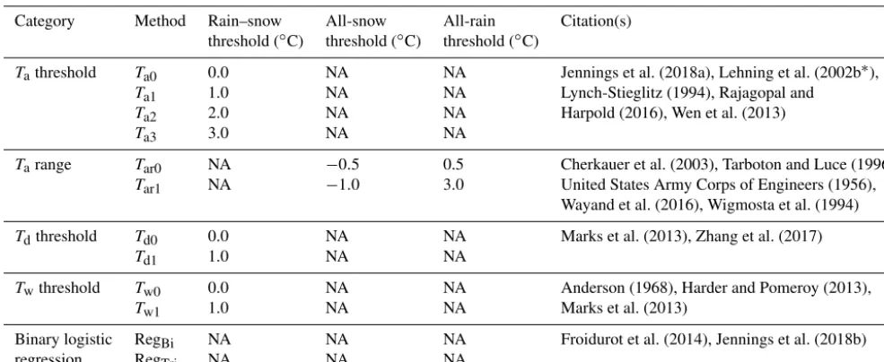
crit-Table 2. Details on the precipitation phase methods used in this work. The temperature value for each threshold method is given in the “Rain–snow threshold” column. The “All-snow threshold” and “All-rain threshold” columns, respectively, give theTavalues below which all precipitation is snow and above which all precipitation is rain for theTarange methods. The regression models compute phase as a function of meteorological conditions (Eqs. 1 and 2) during precipitation and are not associated with a threshold value. Due to a large variety of precipitation thresholds and ranges (Feiccabrino et al., 2015; Harpold et al., 2017b; Jennings et al., 2018b), the citations are listed if the values are approximate. NA: not available.

Category Method Rain–snow All-snow All-rain Citation(s) threshold (◦C) threshold (◦C) threshold (◦C)

Tathreshold Ta0 0.0 NA NA Jennings et al. (2018a), Lehning et al. (2002b∗), Ta1 1.0 NA NA Lynch-Stieglitz (1994), Rajagopal and

Ta2 2.0 NA NA Harpold (2016), Wen et al. (2013)

Ta3 3.0 NA NA

Tarange Tar0 NA −0.5 0.5 Cherkauer et al. (2003), Tarboton and Luce (1996), Tar1 NA −1.0 3.0 United States Army Corps of Engineers (1956),

Wayand et al. (2016), Wigmosta et al. (1994)

Tdthreshold Td0 0.0 NA NA Marks et al. (2013), Zhang et al. (2017)

Td1 1.0 NA NA

Twthreshold Tw0 0.0 NA NA Anderson (1968), Harder and Pomeroy (2013),

Tw1 1.0 NA NA Marks et al. (2013)

Binary logistic RegBi NA NA NA Froidurot et al. (2014), Jennings et al. (2018b)

regression RegTri NA NA NA

∗_{The SNOWPACK default is a 1.2}◦_CT

athreshold.

ical examination of these methods should be made as well. However, such an analysis is beyond the scope of the current work.

3.3 Evaluating the effect of precipitation phase method selection on snowfall fraction and simulated snow cover evolution

For water years (WY; 1 October of the previous calendar year to 30 September) 2004–2011, we simulated snowpack accumulation and melt at the 11 stations using the SNOW-PACK model. Each station had a total of 12 unique model runs corresponding to the different precipitation phase meth-ods. All forcing data and the model setup remained the same across the runs at each site except for the precipitation phase method. For each site and for each of the different pre-cipitation phase methods we quantified the average annual snowfall fraction, peak SWE magnitude, the timing of peak SWE, snowmelt rate, and snow cover duration (Fig. 2). For this work, snowmelt rate is computed as the daily average snowmelt rate between peak SWE timing and the first day where SWE=0 mm. Snow cover duration is the total num-ber of days when simulated SWE is greater than zero. For each of the sites we present the average simulated quanti-ties noted above as well as the range and relative differences of snow metrics associated with the different precipitation phase methods. In this work, the relative difference is defined as the percentage difference between the maximum and min-imum snow metric value (e.g., if Ta0produced a minimum

peak SWE of 200 mm andTa3 produced a maximum peak SWE of 400 mm, the relative difference would be 100 %). Stations with greater variability in their snow cover evolution metrics were considered to be more sensitive to the choice of precipitation phase method.

3.4 Computing the effect of deviating from an optimized rain–snowTathreshold

We were interested in identifying an optimized rain–snow

Tathreshold for our study sites despite a lack of direct pre-cipitation phase observations. We did this through the use of several data sources: (1) the spatially continuous rain– snowTathreshold map from Jennings et al. (2018b), (2) the observed rain–snow Ta threshold (Jennings et al., 2018b) from the measurement location closest to each study site, (3) changes in observed SWE, and (4) changes in observed snow depth at each site to infer snowfall. For 3 and 4, we used a modified version of the approach of Rajagopal and Harpold (2016) to predict precipitation phase by designat-ing a daily increase of SWE or snow depth as snowfall and a zero change or decrease as rainfall when precipitation was greater than 2.54 mm and SWE or snow depth was greater than 0 mm. We then binned snowfall frequency per 1◦CTa bin and computed the rain–snowTathreshold using the hy-perbolic tangent equation of Dai (2008). Thresholds from 1, 2, 3, and 4 were then arithmetically averaged and rounded to the nearest integer value to produce an optimized rain–snow

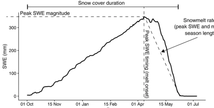
Figure 2.Example plot showing seasonal snow cover evolution, adapted from Trujillo and Molotch (2014).

threshold values in Table 2. Following this step, we evaluated the effect of deviating by±1◦C from the optimized threshold by quantifying differences in peak SWE, peak SWE timing, snow cover duration, and snowmelt rate across the selected thresholds.

3.5 Evaluating the relationships between climate and snow cover sensitivity

In addition to quantifying the variability introduced by the different precipitation phase methods, we evaluated the con-trol exerted by daily meteorology and seasonal climate on snow cover evolution sensitivity at our study sites. We first examined how daily average Ta and RH introduced vari-ability into the simulated snowfall fraction. We did this by grouping all daily meteorological conditions in 1◦CTabins from−8 to+8◦C and 10 % RH bins from 60 % to 100 % on days with precipitation. We then calculated the standard de-viation in the daily snowfall fraction within each bin across all sites and methods. Those results were used to determine theTarange that produced the greatest standard deviation in the daily snowfall fraction. Next, we computed the propor-tion of December–May (i.e., winter and spring) precipitapropor-tion that fell within thatTarange at each site for each simulation year and used that percentage to predict the annual snow-fall fraction range with ordinary least-squares regression. Fi-nally, we evaluated how December–MayTaand precipitation produced variability in peak SWE by plotting the peak SWE range as a function of the two meteorological quantities and plotting a predictive surface with a loess function.

4 Results

4.1 Model validation

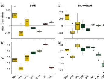
Figure 3 displays the mean bias andr2 values for the dif-ferent precipitation phase methods relative to observations of SWE and snow depth, aggregated across all stations with a given validation measurement. In terms of mean bias, the binary regression models, RegBiand RegTri, as well as the

Ta1 threshold provided the best performance, with average values between 3.1 and 9.1 mm compared to observed SWE and between 4.9 and 14.5 mm compared to observed snow depth. Conversely, theTa0,Ta2, andTa3thresholds and the

Tar0range provided the worst performance, withTa2andTa3 overpredicting andTa0andTar0underpredicting snow accu-mulation by upwards of 100 mm relative to observed SWE and 200 mm and greater relative to observed snow depth. There was relatively little divergence inr2values across the methods, with differences of only 0.07 and 0.08 between the maximum and minimum average r2 values for SWE and snow depth, respectively. The lowest r2 values were pro-duced by theTa0 threshold andTar0range, while Td1,Tw1, and the higherTathresholds produced the highest values.

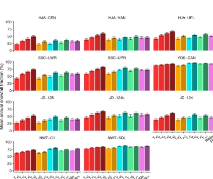
Figure 4 presents model performance relative to observed SWE and snow depth at the different sites. Mean biases were lowest at the NWT stations and at SSC-UPR relative to SWE observations and at the JD stations and SSC-LWR relative to snow depth observations. Averager2values were between 0.65 and 0.91 for SWE, except at NWT-SDL (0.52) and HJA-VAN (0.51), and 0.61 and 0.79 for snow depth, except at JD-124 (0.46).

4.2 Mean simulated snow cover properties

Figure 3.Mean bias(a, c)andr2(b, d)values for the SNOWPACK simulations relative to observed SWE(a, b)and snow depth(c, d). The boxplots show the median, interquartile range, minimum, maximum, and outlying values for each objective function for the different precipitation phase methods at all stations. The open triangles indicate the mean objective function value for that precipitation phase method at all stations.

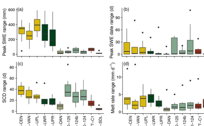
deviation of the given snow metric using all 12 simula-tions at each station, where each simulation corresponded to a different precipitation phase method. Mean peak SWE ranged from 73.1 mm at JD-124 to 1146.1 mm at HJA-UPL. The date of peak SWE, or melt onset, also displayed large variability, with values ranging from 24 January at JD-125 to 13 May at NWT-SDL. Melt rates were all greater than 10 mm d−1during the ablation season except for the JD sta-tions, and the greatest melt rates were simulated at HJA-UPL and SDL. Snow cover duration was greatest at NWT-SDL at 241.1 d, while snow cover was simulated for less than 3 months, on average, at JD-125 and JD-124.

4.3 Effect of precipitation phase method on simulated snowfall fraction

Average annual snowfall fraction (all methods and all years) ranged from 32.3 % at the HJA-CEN station to 92.4 % at the YOS-DAN station (Table 4; Fig. 5). In this case, more strongly seasonal precipitation at YOS-DAN (Table 1) pro-duced a higher annual snowfall fraction than NWT-SDL de-spite the former station’s warmer averageTa. YOS-DAN and NWT-SDL also had the lowest ranges, at 10.1 % and 10.3 %, respectively, suggesting that precipitation phase method se-lection was less important relative to the other stations. Con-versely, the range in the annual snowfall fraction simulated by the different methods was greater than 18 % at all remain-ing stations, reachremain-ing a maximum of 32.3 % at SSC-LWR. For all sites except YOS and NWT, relative differences were greater than 30 %. In some years at HJA, SSC, and JD, the relative difference between the minimum annual snowfall fraction and the maximum exceeded 100 %, meaning that the methods producing the most snow simulated more than dou-ble the annual snowfall fraction of those producing the most rainfall. The greatest relative difference in the annual snow-fall fraction of 126.9 % was simulated at HJA-CEN, more than 10 times greater than at YOS-DAN and NWT-SDL.

4.4 Effect of precipitation phase method on simulated snow accumulation and melt

There were marked differences between the stations in terms of the effect that precipitation phase method choice had on seasonal snow cover evolution. Figure 6 presents the simu-lated mean daily SWE of all simulation years at the study stations along with the difference between the minimum and maximum mean daily SWE produced by the precipitation phase methods. At HJA, SSC, and JD, differences increased throughout the accumulation period, reaching a maximum after peak SWE during the snowmelt season. At NWT and YOS, the differences were typically negligible throughout the accumulation season, as cold winter and early spring tem-peratures produced little divergence in the amount of snow-fall versus rainsnow-fall simulated by the different methods. At these stations, differences in the mean daily SWE produced

by the precipitation phase methods did not appear until ap-proximately the date of peak SWE. Mean daily SWE differ-ences were always less than 90 mm at NWT and YOS, while they sometimes exceeded 200 mm at HJA and SSC. Differ-ences were typically small in magnitude at JD but were pro-portionally large due to low mean daily SWE values.

Breaking down the analysis to the individual snow cover evolution metrics reveals more differences in the sensitivity of the sites to precipitation phase method selection (Fig. 7). In terms of the peak SWE range, the HJA and SSC stations were most sensitive, with average ranges all greater than 200 mm, exceeding 400 mm in some years (Fig. 7a). Con-versely, YOS and NWT were relatively insensitive, as their average ranges were all less than 65 mm. The largest annual range in peak SWE at the NWT and YOS stations was just 90.8 mm at NWT-C1, which was considerably less than the maximum peak SWE range of 592.5 mm simulated at HJA-UPL. Although the JD stations showed little sensitivity in terms of range with average annual peak SWE differences being less than 55 mm, they expressed significant sensitivity when looking at relative differences (Table 5) due to their low mean annual peak SWE (Table 3). Thus, percentage-wise, JD was as sensitive as the two warm maritime sites to the selec-tion of a precipitaselec-tion phase method. At JD, HJA, and SSC it was common for the relative difference between minimum and maximum modeled peak SWE to be well above 50 %, meaning that a significant proportion of water was simulated to have infiltrated or run off using one precipitation phase method versus being stored in the snowpack using another method. This is in stark contrast to the 4.0 % and 1.8 % rela-tive differences at YOS-DAN and NWT-SDL.

JD and HJA were also sensitive to precipitation phase method selection in terms of peak SWE date (Fig. 7b), with four of the six stations having average ranges greater than 2 weeks. In some simulation years, peak SWE date ranges exceeded 1 month at HJA, JD, and SSC. We found that the greatest differences in peak SWE dates were generally sim-ulated on years with low or transient snow cover. In these cases, late-season precipitation was simulated as rain by the lowTathresholds and snow by the highTathresholds, mean-ing that an early SWE maximum was recorded as the peak in the former case and a late SWE maximum in the latter case. Compared to the other stations, peak SWE date ranges were generally small at NWT-SDL and YOS-DAN, with an aver-age range of just 0.8 d at the former and 2.5 d at the latter.

Table 3.Mean snow cover evolution metrics for the 11 stations. Each mean and standard deviation was calculated across all water years and all precipitation phase methods.

Peak SWE Peak SWE date Melt rate SCD (d)

(mm) (mm d−1)

Station Mean SD Mean SD (d) Mean SD Mean SD

HJA-CEN 522.7 252.9 16 February 22.0 15 3.9 158.4 28.2 HJA-VAN 643.1 305.9 14 February 22.2 14.5 3.2 173.1 27.9 HJA-UPL 1146.1 469.9 14 March 23.0 24.9 7.3 201.1 22.4 SSC-LWR 531.9 160.1 8 March 19.0 17.6 3.6 145.6 27.8 SSC-UPR 617.9 298.8 5 March 26.6 17.6 6.0 149.2 35.6 YOS-DAN 674.4 236.7 18 March 17.5 10.9 4.1 208.2 40.3 JD-125 83.4 46.5 24 January 28.5 4 1.5 78.1 31.5 JD-124b 177.5 87.6 1 February 25.8 5.7 2.5 122.4 23.9 JD-124 73.1 35.0 2 February 31.4 3.5 2.8 77.6 30.7 NWT-C1 407.2 78.5 22 April 10.8 11.9 2.8 225.3 19.2 NWT-SDL 915 234.2 13 May 10.0 24.4 10.1 241.1 14.9

Figure 6.Mean daily simulated SWE (solid black line) and the difference between maximum and minimum mean daily SWE (shading) at the study stations. The mean daily SWE was computed by averaging the simulated SWE on each day for all precipitation phase methods across the simulation years. The difference was calculated by subtracting the minimum mean daily SWE from the maximum mean daily SWE produced by the different precipitation phase methods (mean daily SWE plots broken out by precipitation phase method can be viewed in Figs. S1–S11). TheTa0andTar0methods typically produced the minimum mean daily SWE, whileTa3andTd1produced the maximum.

Figure 7.The annual range in simulated peak SWE(a), peak SWE date(b), snow cover duration(c), and melt rate(d)due to precipitation phase method selection at the study stations.

simulated snow cover was typically of a shorter duration compared to the other sites (Table 3). The average relative difference at JD-125 of 120.4 % meant that snow cover sim-ulated using theTa3 threshold lasted twice as long as snow cover using theTa0threshold. Notably, there was an order of magnitude of difference between JD, HJA, and SSC and YOS and NWT, with average relative differences in snow cover duration being greater than 10 % at the former three sites and less than 10 % at the latter two.

Table 4. Statistics for average annual snowfall fraction computed using the different precipitation phase methods across all simulation years at the 11 study stations. The range was calculated by subtract-ing the lowest average annual snowfall fraction from the highest average annual snowfall fraction at each station. The relative differ-ence was then computed as the range divided by the minimum and multiplied by 100 %.Ta0andTar0typically produced the lowest av-erage annual snowfall fractions, whileTa3andTd1led to the highest average annual snowfall fractions.

Annual snowfall fraction (%)

Station Average Range Relative difference

HJA-CEN 32.3 27.4 126.9

HJA-VAN 45.5 22.6 61.1

HJA-UPL 51.8 25.7 62.3

SSC-LWR 56.8 32.3 76.7

SSC-UPR 71.2 25.0 42.8

YOS-DAN 92.4 10.1 11.6

JD-125 39.1 26.0 97.1

JD-124b 55.7 23.2 51.8

JD-124 47.9 23.9 63.6

NWT-C1 70.4 18.2 29.7

NWT-SDL 82.4 10.3 13.4

Table 5.Average relative differences in annual peak SWE, snow cover duration, and melt rate at the 11 stations. Relative differences were not computed for peak SWE date because the relative differ-ence value would change depending on if day of year or day of water year were used in the calculation.

Average relative difference (%)

Station Peak SWE SCD Melt rate

HJA-CEN 86.6 28.0 33.2

HJA-VAN 55.2 19.6 27.5

HJA-UPL 49.1 15.4 19.6

SSC-LWR 78.6 14.9 26.7

SSC-UPR 43.9 13.4 15.6

YOS-DAN 4.0 4.8 11.5

JD-125 74.6 120.4 220.2

JD-124b 54.7 28.7 47.8

JD-124 71.9 72.4 235.5

NWT-C1 16.9 7.0 26.0

NWT-SDL 1.8 1.9 13.0

that the forcing data were kept constant for the different mod-eling scenarios – only the precipitation phase methods were varied. Thus, any changes to the melt rate were caused by shifts in snowmelt timing and by the hydrologic and energy balance impacts of rain versus snow.

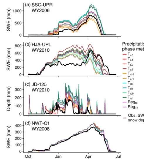
To close this section, it is useful to visualize what these differences look like in terms of annual snow cover evolu-tion. Figure 8 shows examples of large ranges in peak SWE (Fig. 8a), peak SWE date and melt rate (Fig. 8b), and snow

Figure 8.Example simulation years from a selection of stations showing pronounced differences in peak SWE magnitude(a), peak SWE date and snowmelt rate (b), and snow cover duration (c). Panel(d)exemplifies a site and year with little divergence in the studied snowpack metrics. In all panels simulated SWE and snow depth are represented by colored lines for the different methods, while observed SWE and snow depth are shown in black.

4.5 The effect of deviating from an optimized rain–snowTathreshold

Using the data outlined in Sect. 3.4, we identified optimized rain–snowTathresholds of 1.0◦C for HJA and SSC, 2.0◦C for YOS-DAN and JD, and 3.0◦C for NWT (for all snowfall frequency curves and threshold values, please see Figs. S12 and S13 and Table S2). Again, we rounded to the nearest in-teger value to be consistent with the otherTathresholds stud-ied in this work. Consistent with our findings in Sect. 4.4, the warm maritime HJA and SSC stations were profoundly affected by deviations from the optimized threshold (Fig. 9). Differences at these sites produced by deviating by only

±1◦C from the optimized thresholds range between 141 and 403 mm for peak SWE, 1 and 16 d for peak SWE day of wa-ter year (DOWY), and 9 and 29 d for snow cover duration (SCD). Compare this to 1 to 10 mm for peak SWE, 0 to 1 d for peak SWE DOWY, and 1 to 5 d for SCD at the YOS and NWT stations. The consistent story is again that threshold choice makes a much larger impact at a warm site relative to a cold one.

4.6 Climatic controls on precipitation phase method sensitivity

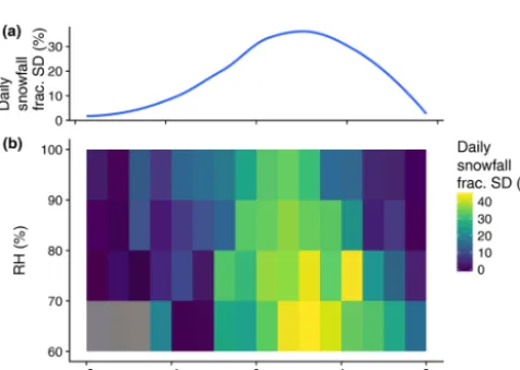
In general, the daily snowfall fraction standard deviation was greatest at daily Ta values between 0 and 4◦C (Fig. 10a). RH provided a secondary control, with greater daily snow-fall fraction variability at lower RH values (Fig. 10b). Over-all, the largest standard deviations in snowfall fraction were simulated at a daily RH less than 80 % andTabetween 1 and 3◦_{C. However, it should be noted that 75.2 % of all}

precip-itation recorded at the study stations occurred in the 90 %– 100 % RH bin. Therefore, although daily snowfall fraction standard deviations were highest at lower RH values, the ma-jority of the variability in snowfall fraction was an effect of

Ta. In this context, the percentage of December–May precip-itation that fell within the 0–4◦CTarange explained 80.1 % of the variance in the annual snowfall fraction range across the study sites (Fig. 11).

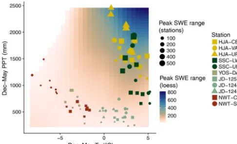
We next evaluated how sensitivity in peak SWE was re-lated to seasonal climate. In this case, warmer Ta and in-creased PPT were both associated with greater ranges in the peak SWE simulated by the different precipitation phase methods (Fig. 12). This meant that the maritime sites HJA and SSC had the greatest sensitivity to the precipitation phase method due to their relatively warmTaand high PPT values. Conversely, moderate PPT values and lowerTa led to mini-mal sensitivity at the cold continental NWT stations and the cold maritime YOS-DAN station. Again, the effect ofTaon sensitivity was manifest in the data. In high snowfall years at NWT-SDL, December–May PPT approached that of the low December–May PPT years at HJA and SSC. However, despite the increased PPT at NWT-SDL, the range in peak

SWE predicted by the different precipitation phase methods remained low.

5 Discussion

5.1 A best precipitation phase method?

In this work we showed that the selection of a precipita-tion phase method produces varying degrees of variability in modeled snow accumulation and melt at our study stations. The different methods also expressed variable performance relative to observations of SWE and snow depth, with the bi-nary regression models, RegBiand RegTri, as well as theTa1 threshold producing the lowest biases (Fig. 3). Previous ob-servational work has shown that, in general, methods incor-porating humidity information outperformTa-only methods when it comes to predicting precipitation phase (Harder and Pomeroy, 2013; Jennings et al., 2018b; Marks et al., 2013; Ye et al., 2013). The RegBimethod, which predicts phase as a function ofTaand RH, exceeded all other methods in par-titioning rain and snow in a Northern Hemisphere precipita-tion phase method comparison (Jennings et al., 2018b). Our study showed that RegBialso typically produced simulations of SWE and snow depth that had low biases relative to ob-servations (Fig. 3) and led to snow cover evolution metrics that were neither extremely high nor low compared to the other methods examined in this work. This finding is com-plemented by the performance of other humidity-based met-rics, which produced average SWE and snow depth biases between−19.2 and 25.1 and−58.3 and 56.7 mm, respec-tively.

This is in contrast to theTathresholds and ranges, which produced the largest magnitude biases. Notably, the four worst performers were theTa0,Tar0,Ta2, and Ta3 methods, with the former two underpredicting snow accumulation and the latter two overpredicting it. Across our study sites, the onlyTamethods that performed well relative to observations were theTa1threshold andTar1range. These modeling results confirm again that including humidity information, whether it is in the form of a binary logistic regression model,Tw, or

Td, offers advantages over aTa-only method. It is important to note again that we chose methods that covered the range in rain–snow partitioningTavalues across our study domain or that included humidity information. The only methods not falling into this category wereTa0andTar0, which were cho-sen because they are still employed as default methods in some models and studies. Although there are some small ge-ographic regions where such a threshold or range may be appropriate (Jennings et al., 2018b), they are unsuitable for many locations and should not be used for large-scale stud-ies.

Figure 9.Mean peak SWE(a), peak SWE day of water year (DOWY;b), snow cover duration (SCD;c), and melt rate(d)for the different stations. The width of the bar in each plot represents the spread between the mean snow cover metric value when the model was run with the optimized threshold plus 1◦C and the optimized threshold minus 1◦C. The center line represents the snow cover metric value when the model was run with the optimized threshold. Note: at NWT, only−1◦C from the optimized value of 3◦C was evaluated because we did not include a 4◦C threshold in this work.

Figure 10. The standard deviation of daily snowfall fraction as a function ofTa(a)and as a function ofTaand RH(b). We binned the meteorological quantities within the ranges shown and calcu-lated the standard deviation of snowfall fraction perTabin (a) and Ta/RH bin(b)using simulated precipitation phase from all stations and all methods.

(Fig. 3). This suggests that the ranges and the mixed-phase precipitation they produced provided little further informa-tion on precipitainforma-tion phase at the hourly model timescale rel-ative to the thresholds. However, it should be noted there are relatively few quantitative data on the frequency and solid–liquid proportions of mixed-phase events (e.g., Yuter et al., 2006). Work from the Turin region of Italy showed that mixed-phase events are relatively few compared to all-rain and all-snow events (Avanzi et al., 2014), while research in a maritime climate indicated that mixed-phase events can be quite frequent (Wayand et al., 2016). Future work would therefore benefit from further explorations of the frequency

Figure 11.Range in annual snowfall fraction as predicted by the proportion of December–May PPT falling between 0 and 4◦C. Each point represents one simulation year at a station identified by the color and shape. The black line of best fit was calculated using or-dinary least-squares regression (r2=0.80;pvalue<0.0001).

of mixed-phase events and model representations thereof at multiple timescales.

opti-Figure 12.Range in annual peak SWE as simulated by the differ-ent precipitation phase methods at the 11 study stations. Each point represents one simulation year at a given station, and larger points correspond to larger differences in maximum minus minimum peak SWE. The background shading corresponds to ranges in peak SWE predicted by a loess function fit to the station data.

mized model setups at each site but rather kept the model setup consistent in order to compare the sensitivity of phase partitioning without introducing other uncertainties. Thus, the lowr2and higher bias values at HJA-VAN, NWT-SDL, and JD-124 (Fig. 4) could likely be improved with model tuning, but we did not pursue such an approach. Addition-ally, we showed in Sect. 4.5 that deviating from an optimized

Tarain–snow threshold by±1◦C had a much larger effect on simulated snow accumulation and melt at HJA and SSC than YOS and NWT. Such a finding indicates that finding an op-timal threshold is much more important in areas with winter

Tanear freezing.

5.2 Assumptions and limitations

Snow modeling studies are hindered by inherent uncertain-ties in model structure (Essery et al., 2013; Etchevers et al., 2004; Rutter et al., 2009; Slater et al., 2001) and forcing data (Lapo et al., 2015; Raleigh et al., 2015, 2016). While the research presented herein shows that the precipitation phase method should be considered another critical com-ponent of model uncertainty, our work was also likely af-fected by the aforementioned issues in structure and forcing data which can be seen in the variability in model perfor-mance at the different sites (Fig. 4). In this work, we used the well-validated, physics-based SNOWPACK model, but past research has shown that there is no best snow model and that model performance varies both within and across study sites (e.g., Rutter et al., 2009). Given this variable perfor-mance and differences in snow model structure and physics, it is possible that some models may be more or less sensitive to the choice of a precipitation phase method. Our use of a single model may overestimate or underestimate the sensi-tivity of snow accumulation and melt to precipitation phase

method selection. Future research should therefore focus on how model choice affects the sensitivity of simulated snow cover evolution to the precipitation phase method.

In addition to the uncertainties introduced by the SNOW-PACK model, we used empirical methods to estimateTdand

Tw, which could affect rain–snow partitioning. We were sat-isfied with the performance of theTdmethod, as it strongly matched Td observations from JD (Sect. 3.2). However, there were no observations ofTw on which to validate the Stull (2011) method, which was optimized for standard sur-face pressure and for a range ofTaand RH values. The fig-ures in Stull (2011) show that pressure-induced uncertainty inTw is generally less than 1◦C when RH >50 %. Addi-tionally, the total percentage of precipitation observations falling within the Stull (2011)Ta and RH ranges was be-tween 94.3 % and 100 % at our stations. Thus, we expect only marginal uncertainty to be introduced by the empirical meth-ods. However, precipitation phase and hydrometeor temper-ature are strongly related toTw(Harder and Pomeroy, 2013), suggesting that there should be enhanced monitoring ofTw at research sites.

Furthermore, our research only examined methods that partition precipitation phase using surface meteorological quantities such asTa, RH, andPs. Atmospheric and climate models can also be used for hydroclimatic simulations either through direct coupling in earth system models or as forcing data for land surface models. Many such models employ mi-crophysics schemes to assign and track precipitation phase from the formation of a hydrometeor, through various atmo-spheric layers, to the land surface. For example, the Weather Research and Forecasting (WRF) model (Skamarock et al., 2005) has been used to simulate snow cover accumulation and ablation over large study domains in the western United States when coupled to a land surface model (Ikeda et al., 2010; Musselman et al., 2017a; Rasmussen et al., 2011). WRF has also been used to model the elevation of the rain– snow transition line in order to evaluate which basin areas are receiving solid or liquid precipitation during storm events (Minder et al., 2011). In addition, work from the fifth phase of the Coupled Model Intercomparison Project (CMIP5) has shown that climate models produce different snowfall frac-tions due to variafrac-tions in both climate and the precipitation phase method (Krasting et al., 2013). In CMIP5, some mod-els utilize microphysics schemes, while others assign precip-itation phase at the land surface using methods similar to the ones presented in this work. Therefore, understanding and quantifying the sensitivity of model output due to precipi-tation phase method selection are important for both hydro-logic and climate modeling studies.

5.3 Physical mechanisms controlling sensitivity to phase method

(Fig. 7). These ranges were typically larger than 200 mm and sometimes exceeded 400 mm with relative differences usu-ally greater than 50 %, indicating large uncertainty in snow-pack water storage. Additionally, peak SWE date ranges typ-ically exceeded 2 weeks at these stations, meaning that the timing of snowmelt onset was also affected by the precip-itation phase method. These large variations in snow cover evolution were likely due to the combined effect of reduced frozen mass entering the snowpack and subsequent changes to the snowpack energy balance. For the former, both HJA and SSC had high proportions of precipitation falling be-tween 0 and 4◦C (Fig. 11), which led to wide ranges in the annual snowfall fraction (Table 4). The methods producing lower annual snowfall fractions (e.g.,Ta0andTar0) generally corresponded to reduced snow cover duration simply because there was less frozen mass to melt. In other words, the energy required to melt the entire snowpack was reduced relative to the methods producing higher snowfall fractions, and the snowpack could be melted over a shorter time period.

Compounding the response of the warm maritime sites is the fact that snow and rain have different fates when they enter a snowpack, with resultant effects on the snowpack en-ergy budget. Snowfall can increase snowpack cold content (Jennings et al., 2018a), refresh surface albedo (Clow et al., 2016; Molotch et al., 2004; Molotch and Bales, 2006; Painter et al., 2012; United States Army Corps of Engineers, 1956), and provide dry pore space that must reach field capacity with liquid water before runoff can begin (Bengtsson, 1982; Seligman et al., 2014). Rainfall, conversely, can advect heat to the snowpack (Marks et al., 1998), infiltrate and run off (Harr, 1981, 1986), or be refrozen in the snowpack if there is cold content to be satisfied. In this context, the precipitation phase methods that produced more rainfall likely affected snow cover evolution not just through reduced frozen mass but also through changes to the snowpack energy budget. Further observational and modeling research is warranted to evaluate how rain versus snow affects snowpack energetics.

5.4 Why precipitation phase matters to climate warming simulations

The shift from snow to rain in cold and temperate regions across the globe is expected to continue with further warm-ing. Future air temperature increases will likely produce re-duced snowfall fractions (Klos et al., 2014; Lute et al., 2015; Safeeq et al., 2015), lower peak SWE values (Adam et al., 2009), earlier snowmelt onset (Stewart et al., 2004), slower snowmelt rates (Musselman et al., 2017a), and changes to the intensity and location of rain-on-snow events (Mussel-man et al., 2018). These warming-driven changes will impact both water resource availability (Barnett et al., 2008) and land surface albedo (Déry and Brown, 2007). Most at risk of reductions in the snowfall fraction and snow accumulation are areas with winterTanear 0◦C (Nolin and Daly, 2006). Concerningly, our work shows that it is precisely these

ar-eas that have the greatest modeled snow cover accumulation and melt sensitivity to precipitation phase method selection. Compounding the problem is the fact that all precipitation phase methods exhibit downgraded performance relative to observations between 0◦C and 4◦C (Ding et al., 2014; Jen-nings et al., 2018b).

Harpold et al. (2017c) showed that future changes to snow-fall fraction are moderated or exacerbated by the choice of a precipitation phase method, depending on the area’s relative humidity. However, how this uncertainty affects the conclu-sion of climate change predictions is typically not discussed. In the context of the work presented herein, there should be a focus applied to areas where the baseline variability in peak SWE, snowmelt onset, and snow cover duration due to pre-cipitation phase method approaches or exceeds the simulated change in the associated snowpack properties with warming. In warm maritime climates, research has shown that peak SWE may decrease by upwards of several hundred millime-ters as warming continues (e.g., Cooper et al., 2016; Leung et al., 2004; Minder, 2010; Musselman et al., 2017b), which is near the range of peak SWE sensitivity values reported in this work. Precipitation phase method selection is also likely to impact simulations of future warm snow droughts, where anomalously warm winters are associated with low peak SWE (Harpold et al., 2017a). In addition, snow cover duration variability due to precipitation phase method selec-tion in earth system models may affect simulaselec-tions of the snow–albedo feedback, which is the amplification of surface warming due to reduced snow cover (Hall, 2004; Hall and Qu, 2006). As climate warming shifts new areas towards the winter and spring averageTavalues (0–4◦C) that lead to the greatest uncertainty in rain–snow partitioning, our research suggests that uncertainty in future hydroclimatic states will be exacerbated by precipitation phase method selection.

6 Conclusion

Conversely, the YOS-DAN and NWT-SDL stations exhibited the lowest sensitivity to precipitation phase method selec-tion, with relative differences in the annual snowfall fraction between 11.6 % and 13.4 %. Peak SWE ranges were typi-cally less than 30 mm for these two stations, while average snowmelt onset date ranges were only 0.8 and 2.5 d at YOS-DAN and NWT-SDL, respectively. In contrast to the marked differences in peak SWE, melt onset, and snow cover du-ration between the warm and cold stations, ranges in the snowmelt rate exhibited a small relationship to seasonal cli-mate. Additionally, we found that deviating by±1◦C from an optimizedTa rain–snow threshold had a relatively small effect on simulated snow cover evolution at NWT and YOS compared to the larger sensitivity at HJA, SSC, and JD.

The spatially variable sensitivity of snow cover evolution was primarily a result of climatic differences between the sta-tions. Increased December–MayTaand PPT were associated with greater peak SWE ranges across the different precipita-tion phase methods. This meant that the maritime sites HJA and SSC, with significant winter and spring PPT, were most affected by precipitation phase method selection. Overall, we found stations with a high proportion of December–May PPT falling at Ta between 0 and 4◦C to be more sensitive than those with less PPT in that Ta range. This is troublesome, considering that climate warming is expected to push new areas in the seasonal snow zone towards winterTanear 0◦C and above. It is therefore critical that future work examine the relationship between the effect of warming on snow cover evolution and the model variability that results from precipi-tation phase partitioning uncertainty, particularly in areas un-dergoing a snow-to-rain transition.

Code and data availability. Forcing and validation data can be ac-cessed at the following sites (as of 11 February 2019):

– H.J. Andrews LTER: https://doi.org/10.6073/pasta/ c96875918bb9c86d330a457bf4295cd9 (McKee, 2015) and http://andlter.forestry.oregonstate.edu/data/ (last access: 16 July 2019) (for sub-daily data),

– Southern Sierra CZO: http://criticalzone.org/sierra/data/ dataset/2529/ (last access: 9 September 2019, Husaker, 2011a) and http://criticalzone.org/sierra/data/dataset/2406/ (last access: 9 September 2019, Husaker, 2011b),

– Johnston Draw (Reynolds Creek CZO): https://doi.org/10.15482/USDA.ADC/1402076 (Godsey et al., 2016, 2018),

– Yosemite Dana Meadows: http://hdl.handle.net/1773/35957 (Lundquist et al., 2016),

– Niwot Ridge LTER: https://doi.org/10.6073/pasta/ 1538ccf520d89c7a11c2c489d973b232 (Jennings et al., 2018a, c) and https://doi.org/10.6073/pasta/ f62b0a3741737c871958cf7e63c089e0 (Williams, 2016a, b).

SNOWPACK version 3.4.5 was used for this research. The model source code can be accessed at https://models.slf.ch/ (last access: 9 September 2019). For the code used to automatically run the

model with the different precipitation phase methods and ana-lyze the output data, please contact the corresponding author. The color palettes used in this paper’s figures can be accessed online from their respective authors (https://github.com/karthik/ wesanderson, last access: 9 September 2019, Ram, 2019, and https://doi.org/10.5281/zenodo.1243862, Crameri, 2018).

Supplement. The supplement related to this article is available on-line at: https://doi.org/10.5194/hess-23-3765-2019-supplement.

Author contributions. KSJ and NPM designed the study. KSJ per-formed the analyses and wrote the paper. NPM provided feedback and edited the paper.

Competing interests. The authors declare that they have no conflict of interest.

Acknowledgements. The LTER and CZO networks are funded by the United States National Science Foundation. We offer our thanks to Don Henshaw (H.J. Andrews LTER) and Mohammed Safeeq (Southern Sierra CZO) for their assistance with the respective datasets. We are also grateful for the other dataset providers for making their data freely and easily accessible. Additionally, we thank Bettina Schaefli and Jono Conway along with the editor Markus Hrachowitz for their reviews and feedback that helped im-prove this paper.

Financial support. This research has been supported by NASA (grant no. 16-EARTH16F-378).

Review statement. This paper was edited by Markus Hrachowitz and reviewed by Jonathan Conway and Bettina Schaefli.

References

Adam, J. C., Hamlet, A. F., and Lettenmaier, D. P.: Implications of global climate change for snowmelt hydrology in the twenty-first century, Hydrol. Process., 23, 962–972, 2009.

Alduchov, O. A. and Eskridge, R. E.: Improved Magnus form ap-proximation of saturation vapor pressure, J. Appl. Meteorol., 35, 601–609, 1996.

Anderson, E. A.: Development and testing of snow pack energy bal-ance equations, Water Resour. Res., 4, 19–37, 1968.

Angström, A. K.: A study of the radiation of the atmosphere: based upon observations of the nocturnal radiation during expeditions to Algeria and to California, Smithsonian Institution, Washing-ton, DC, 1915.

Auer Jr., A. H.: The rain versus snow threshold temperatures, Weatherwise, 27, 67–67, 1974.

properties: An Italian case study, Am. J. Clim. Change, 3, 43990, https://doi.org/10.4236/ajcc.2014.31007, 2014.

Barnett, T. P., Adam, J. C., and Lettenmaier, D. P.: Potential impacts of a warming climate on water availability in snow-dominated regions, Nature, 438, 303–309, 2005.

Barnett, T. P., Pierce, D. W., Hidalgo, H. G., Bonfils, C., Santer, B. D., Das, T., Bala, G., Wood, A. W., Nozawa, T., Mirin, A. A., Cayan, D. R., and Dettinger, M. D.: Human-induced changes in the hydrology of the western United States, Science, 319, 1080– 1083, 2008.

Bartelt, P. and Lehning, M.: A physical SNOWPACK model for the Swiss avalanche warning: Part I: numerical model, Cold Reg. Sci. Technol., 35, 123–145, 2002.

Bavay, M. and Egger, T.: MeteoIO 2.4.2: a preprocessing library for meteorological data, Geosci. Model Dev., 7, 3135-3151, https://doi.org/10.5194/gmd-7-3135-2014, 2014.

Bengtsson, L.: The importance of refreezing on the diurnal snowmelt cycle with application to a northern Swedish catch-ment, Hydrol. Res., 13, 1–12, 1982.

Bintanja, R. and Andry, O.: Towards a rain-dominated Arctic, Nat. Clim. Change, 7, 263–267, 2017.

Caine, N.: Streamflow patterns in the alpine environment of North Boulder Creek, Colorado Front Range, Z. Geomorphol., 104, 27– 42, 1996.

Cherkauer, K. A., Bowling, L. C., and Lettenmaier, D. P.: Vari-able infiltration capacity cold land process model updates, Glob. Planet. Change, 38, 151–159, https://doi.org/10.1016/S0921-8181(03)00025-0, 2003.

Clow, D. W., Williams, M. W., and Schuster, P. F.: In-creasing aeolian dust deposition to snowpacks in the Rocky Mountains inferred from snowpack, wet deposition, and aerosol chemistry, Atmos. Environ., 146, 183–194, https://doi.org/10.1016/j.atmosenv.2016.06.076, 2016.

Cooper, M. G., Nolin, A. W., and Safeeq, M.: Testing the re-cent snow drought as an analog for climate warming sensitiv-ity of Cascades snowpacks, Environ. Res. Lett., 11, 084009, https://doi.org/10.1088/1748-9326/11/8/084009, 2016.

Crameri, F.: Scientific colour maps (Version 4.0.0), Zenodo, https://doi.org/10.5281/zenodo.2649252, 2018.

Crawford, T. M. and Duchon, C. E.: An improved parameterization for estimating effective atmospheric emissivity for use in calcu-lating daytime downwelling longwave radiation, J. Appl. Meteo-rol., 38, 474–480, 1999.

Dai, A.: Temperature and pressure dependence of the rain-snow phase transition over land and ocean, Geophys. Res. Lett., 35, L12802, https://doi.org/10.1029/2008GL033295, 2008. Deardoff, J. W.: Efficient prediction of ground surface temperature

and moisture with inclusion of a layer of vegetation., J. Geophys. Res., 38, 659–661, 1978.

Déry, S. J. and Brown, R. D.: Recent Northern Hemi-sphere snow cover extent trends and implications for the snow-albedo feedback, Geophys. Res. Lett., 34, L22504, https://doi.org/10.1029/2007GL031474, 2007.

Dickerson-Lange, S. E., Gersonde, R. F., Hubbart, J. A., Link, T. E., Nolin, A. W., Perry, G. H., Roth, T. R., Wayand, N. E., and Lundquist, J. D.: Snow disappearance timing is dominated by forest effects on snow accumulation in warm winter climates of the Pacific Northwest, United States, Hydrol. Process., 31, 1846– 1862, https://doi.org/10.1002/hyp.11144, 2017.

Dilley, A. C. and O’Brien, D. M.: Estimating downward clear sky long-wave irradiance at the surface from screen temperature and precipitable water, Q. J. Roy. Meteor. Soc., 124, 1391–1401, 1998.

Ding, B., Yang, K., Qin, J., Wang, L., Chen, Y., and He, X.: The dependence of precipitation types on surface elevation and me-teorological conditions and its parameterization, J. Hydrol., 513, 154–163, 2014.

Erickson, T. A., Williams, M. W., and Winstral, A.: Persistence of topographic controls on the spatial distribution of snow in rugged mountain terrain, Colorado, United States, Water Resour. Res., 41, W04014, https://doi.org/10.1029/2003WR002973, 2005. Essery, R., Morin, S., Lejeune, Y., and Ménard, C.: A

comparison of 1701 snow models using observations from an alpine site, Adv. Water Resour., 55, 131–148, https://doi.org/10.1016/j.advwatres.2012.07.013, 2013. Etchevers, P., Martin, E., Brown, R., Fierz, C., Lejeune, Y., Bazile,

E., Boone, A., Dai, Y.-J., Essery, R., Fernandez, A., Gusev, Y., Jordan, R., Koren, V., Kowalczyk, E., Nasonova, N. O., Pyles, R. D., Schlosser, A., Shmakin, A. B., Smirnova, T. G., Strasser, U., Verseghy, D., Yamazaki, T., and Yang, Z.: Validation of the energy budget of an alpine snowpack simulated by several snow models (SnowMIP project), Ann. Glaciol., 38, 150–158, 2004. Fassnacht, S. R. and Soulis, E. D.: Implications during transitional

periods of improvements to the snow processes in the land sur-face scheme-hydrological model WATCLASS, Atmos.-Ocean, 40, 389–403, 2002.

Fassnacht, S. R., Venable, N. B. H., Khishigbayar, J., and Cherry, M. L.: The Probability of Precipitation as Snow Derived from Daily Air Temperature for High Elevation Areas of Colorado, United States, Cold and Mountain Region Hydrological Systems Under Climate Change: Towards Improved Projections, in: Pro-ceedings of symposium H02, IAHS-IAPSO-IASPEI Assembly, IAHS, Gothenburg, Sweden, July 2013, 360, 65–70, 2013. Feiccabrino, J., Graff, W., Lundberg, A., Sandström, N.,

and Gustafsson, D.: Meteorological Knowledge Use-ful for the Improvement of Snow Rain Separation in Surface Based Models, Hydrology, 2, 266–288, https://doi.org/10.3390/hydrology2040266, 2015.

Flerchinger, G. N., Xaio, W., Marks, D., Sauer, T. J., and Yu, Q.: Comparison of algorithms for incoming atmo-spheric long-wave radiation, Water Resour. Res., 45, W03423, https://doi.org/10.1029/2008WR007394, 2009.

Froidurot, S., Zin, I., Hingray, B., and Gautheron, A.: Sensi-tivity of Precipitation Phase over the Swiss Alps to Differ-ent Meteorological Variables, J. Hydrometeorol., 15, 685–696, https://doi.org/10.1175/JHM-D-13-073.1, 2014.

Gjertsen, U. and Ødegaard, V.: The water phase of pre-cipitation – a comparison between observed, esti-mated and predicted values, Atmos. Res., 77, 218–231, https://doi.org/10.1016/j.atmosres.2004.10.030, 2005.

Godsey, S. E., Marks, D., Kormos, P. R., Seyfried, M. S., Enslin, C. L., Winstral, A. H., McNamara, J. P., and Link, T. E.: Eleven years of mountain weather, snow, soil moisture and streamflow data from the rain-snow transition zone - the Johnston Draw catchment, Reynolds Creek Experimental Watershed and Critical Zone Observatory, USA, Earth Syst. Sci. Data, 10, 1207-1216, https://doi.org/10.5194/essd-10-1207-2018, 2018.

Greenland, D.: The climate of Niwot Ridge, front range, Colorado, USA, Arct. Alp. Res., 21, 380–391, 1989.

Hall, A.: The Role of Surface Albedo Feedback in Cli-mate, J. CliCli-mate, 17, 1550–1568, https://doi.org/10.1175/1520-0442(2004)017<1550:TROSAF>2.0.CO;2, 2004.

Hall, A. and Qu, X.: Using the current seasonal cycle to constrain snow albedo feedback in future climate change, Geophys. Res. Lett., 33, L03502, https://doi.org/10.1029/2005GL025127, 2006. Harder, P. and Pomeroy, J.: Estimating precipitation phase using a psychrometric energy balance method, Hydrol. Process., 27, 1901–1914, https://doi.org/10.1002/hyp.9799, 2013.

Harder, P. and Pomeroy, J. W.: Hydrological model uncertainty due to precipitation-phase partitioning methods, Hydrol. Process., 28, 4311–4327, 2014.

Harpold, A. A., Dettinger, M., and Rajagopal, S.: Defining snow drought and why it matters, EOS-Earth Space Sci. News, 98, https://doi.org/10.1029/2017EO068775, 2017a.

Harpold, A. A., Kaplan, M. L., Klos, P. Z., Link, T., Mc-Namara, J. P., Rajagopal, S., Schumer, R., and Steele, C. M.: Rain or snow: hydrologic processes, observations, predic-tion, and research needs, Hydrol. Earth Syst. Sci., 21, 1–22, https://doi.org/10.5194/hess-21-1-2017, 2017b.

Harpold, A. A., Crews, J. B., Rajagopal, S., Winchell, T., and Schumer, R.: Relative Humidity Has Uneven Effects on Shifts From Snow to Rain Over the Western U.S., Geophys. Res. Lett., 44, 2017GL075046, https://doi.org/10.1002/2017GL075046, 2017c.

Harr, R. D.: Some characteristics and consequences of snowmelt during rainfall in western Oregon, J. Hydrol., 53, 277–304, 1981. Harr, R. D.: Effects of clearcutting on rain-on-snow runoff in west-ern Oregon: A new look at old studies, Water Resour. Res., 22, 1095–1100, 1986.

Husaker, C.: CZO Dataset: Met Stations, Providence, Lower – Meteorology (2002–2011), available at: http://criticalzone.org/ sierra/data/dataset/2529/ (last access: 9 September 2019), 2011a. Husaker, C.: CZO Dataset: Met Stations, Providence, Upper– Mete-orology (2002-2011), available at: http://criticalzone.org/sierra/ data/dataset/2406/ (last access: 9 September 2019), 2011b. Hunsaker, C. T., Whitaker, T. W., and Bales, R. C.: Snowmelt runoff

and water yield along elevation and temperature gradients in Cal-ifornia’s southern Sierra Nevada, JAWRA J. Am. Water Resour. Assoc., 48, 667–678, 2012.

Ikeda, K., Rasmussen, R., Liu, C., Gochis, D., Yates, D., Chen, F., Tewari, M., Barlage, M., Dudhia, J., and Miller, K.: Simulation of seasonal snowfall over Colorado, Atmos. Res., 97, 462–477, 2010.

Jennings, K. S. and Jones, J. A.: Precipitation-snowmelt timing and snowmelt augmentation of large peak flow events, west-ern Cascades, Oregon, Water Resour. Res., 51, 7649–7661, https://doi.org/10.1002/2014WR016877, 2015.

Jennings, K. S., Kittel, T. G. F., and Molotch, N. P.: Observations and simulations of the seasonal evolution of snowpack cold

con-tent and its relation to snowmelt and the snowpack energy bud-get, The Cryosphere, 12, 1595-1614, https://doi.org/10.5194/tc-12-1595-2018, 2018a.

Jennings, K. S., Winchell, T. S., Livneh, B., and Molotch, N. P.: Spatial variation of the rain-snow temperature threshold across the Northern Hemisphere, Nat. Commun., 9, 1148, https://doi.org/10.1038/s41467-018-03629-7, 2018b.

Jennings, K., Kittel, T., and Molotch, N.: Infilled climate data for C1, Saddle, and D1, 1990– 2013, hourly, Environmental Data Initiative, https://doi.org/10.6073/pasta/1538ccf520d89c7a11c2c489d973b232, 2018c.

Kienzle, S. W.: A new temperature based method to sep-arate rain and snow, Hydrol. Process., 22, 5067–5085, https://doi.org/10.1002/hyp.7131, 2008.

Klos, P. Z., Link, T. E., and Abatzoglou, J. T.: Extent of the rain-snow transition zone in the western US under historic and pro-jected climate, Geophys. Res. Lett., 41, 4560–4568, 2014. Knowles, J. F., Harpold, A. A., Cowie, R., Zeliff, M., Barnard,

H. R., Burns, S. P., Blanken, P. D., Morse, J. F., and Williams, M. W.: The relative contributions of alpine and subalpine ecosystems to the water balance of a mountain-ous, headwater catchment, Hydrol. Process., 29, 4794–4808, https://doi.org/10.1002/hyp.10526, 2015.

Knowles, N., Dettinger, M. D., and Cayan, D. R.: Trends in snowfall versus rainfall in the western United States, J. Climate, 19, 4545– 4559, 2006.

Krasting, J. P., Broccoli, A. J., Dixon, K. W., and Lanzante, J. R.: Future Changes in Northern Hemisphere Snowfall, J. Climate, 26, 7813–7828, https://doi.org/10.1175/JCLI-D-12-00832.1, 2013.

Lapo, K. E., Hinkelman, L. M., Raleigh, M. S., and Lundquist, J. D.: Impact of errors in the downwelling irradiances on simulations of snow water equivalent, snow surface temperature, and the snow energy balance, Water Resour. Res., 51, 1649–1670, 2015. Leavesley, G. H., Restrepo, P. J., Markstrom, S. L., Dixon, M., and

Stannard, L. G.: The Modular Modeling System (MMS): User’s Manual, US Geological Survey, Denver, COOpen File Report 96–151, 1996.

Lehning, M., Fierz, C., and Lundy, C.: An objective snow profile comparison method and its application to SNOWPACK, Cold Reg. Sci. Technol., 33, 253–261, https://doi.org/10.1016/S0165-232X(01)00044-1, 2001.

Lehning, M., Bartelt, P., Brown, B., Fierz, C., and Satyawali, P.: A physical SNOWPACK model for the Swiss avalanche warning: Part II. Snow microstructure, Cold Reg. Sci. Technol., 35, 147– 167, 2002a.

Lehning, M., Bartelt, P., Brown, B., and Fierz, C.: A physical SNOWPACK model for the Swiss avalanche warning: Part III: Meteorological forcing, thin layer formation and evaluation, Cold Reg. Sci. Technol., 35, 169–184, 2002b.

Lehning, M., Völksch, I., Gustafsson, D., Nguyen, T. A., Stähli, M., and Zappa, M.: ALPINE3D: a detailed model of mountain surface processes and its application to snow hydrology, Hydrol. Process., 20, 2111–2128, 2006.