www.hydrol-earth-syst-sci.net/14/765/2010/ doi:10.5194/hess-14-765-2010
© Author(s) 2010. CC Attribution 3.0 License.
Earth System
Sciences
Numerical study of the evaporation process and parameter
estimation analysis of an evaporation experiment
K. Schneider-Zapp1, O. Ippisch2, and K. Roth1
1Institute of Environmental Physics, Heidelberg University, Heidelberg, Germany
2Interdisciplinary Center for Scientific Computing, Heidelberg University, Heidelberg, Germany Received: 3 November 2009 – Published in Hydrol. Earth Syst. Sci. Discuss.: 3 December 2009 Revised: 14 March 2010 – Accepted: 2 May 2010 – Published: 17 May 2010
Abstract. Evaporation is an important process in soil-atmosphere interaction. The determination of hydraulic properties is one of the crucial parts in the simulation of wa-ter transport in porous media. Schneider et al. (2006) devel-oped a new evaporation method to improve the estimation of hydraulic properties in the dry range. In this study we used numerical simulations of the experiment to study the physical dynamics in more detail, to optimise the boundary conditions and to choose the optimal combination of mea-surements. The physical analysis exposed, in accordance to experimental findings in the literature, two different evapora-tion regimes: (i) a soil-atmosphere boundary layer dominated regime (regime I) close to saturation and (ii) a hydraulically dominated regime (regime II). During this second regime a drying front (interface between unsaturated and dry zone with very steep gradients) forms which penetrates deeper into the soil as time passes. The sensitivity analysis showed that the result is especially sensitive at the transition between the two regimes. By changing the boundary conditions it is pos-sible to force the system to switch between the two regimes, e.g. from II back to I. Based on this findings a multistep ex-periment was developed. The response surfaces for all pa-rameter combinations are flat and have a unique, localised minimum. Best parameter estimates are obtained if the evap-oration flux and a potential measurement in 2 cm depth are used as target variables. Parameter estimation from simu-lated experiments with realistic measurement errors with a two-stage Monte-Carlo Levenberg-Marquardt procedure and manual rejection of obvious misfits lead to acceptable results for three different soil textures.
Correspondence to: K. Schneider-Zapp
1 Introduction
Evaporation from porous media is a key process for soil-atmosphere interaction, for example in the coupling with cli-mate or the forcing of lower soil layers, as well as for many industrial and engineering applications. Many investiga-tions are reported in the literature which assess the evapora-tion process. Evaporaevapora-tion from an initially saturated porous medium typically begins with a relatively high drying rate determined primarily by the external forcing. This phase continues as long as the medium can sustain the evapora-tive flow. Then it changes to a stage with falling drying rates (Sherwood, 1930; Scherer, 1990; Shokri et al., 2008). Exten-sive work has been put into pore-scale modelling of the dry-ing process; a review is given by Prat (2002). The pore-scale analysis is valuable for the understanding of the detailed pore-scale processes. However these models typically can-not be directly applied for macroscopic problems, since the actual geometry of the medium is normally not known. On the field scale, many energy-balance based, semi-empirical, or empirical models exist (Foken, 2003). For modelling on the REV scale, in-between the field- and pore-scale, Schnei-der et al. (2006) used a diffusive boundary layer approach coupled with a Richards’ pore space model. It is reasonably simple but still provides a sufficient macroscopic descrip-tion. One aim of this investigation was to further examine the physical implications of that model.
TDR
Tensiometer
atmosphere
boundary layer
p, Tw j [image:2.595.76.259.61.193.2]soil
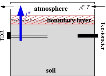
wFig. 1. Sketch of the experimental setup. Evaporation takes place into a gas-tight head space above the soil surface. Air is flowing through it to remove the water. Water vapour molar fraction and temperature in the head space is controlled to define the boundary condition. The water flux is measured by the difference in vapour content of the incoming and outgoing air in a controlled gas flow.
Similar restrictions apply to traditional evaporation experi-ments, where a saturated soil sample is placed on a balance and exposed to free air while the matric potential in several depths is measured by tensiometers. If the potential falls be-low the air-entry value of the tensiometer or bebe-low the vapour pressure of water, whichever is higher, then water is released from the tensiometer into the soil. This leads to a disturbance of the measurements that may be quite dramatic. The mea-surement range is further limited by the technical challenges to measure with tensiometers the very small potential gradi-ents in regions where the hydraulic conductivity is still high, or to assess the little weight change caused by small evapo-ration fluxes in the dry range with a balance.
Schneider et al. (2006) presented a novel evaporation ex-periment which yields reliable data even in the dry and very dry range by measuring the flux at the upper boundary with an infrared absorption gas analyser. An inverse model for the estimation of hydraulic parameters from the evaporation flux was developed. The analysis of an evaporation experiment with an undisturbed soil sample yielded reasonable results.
The objective of this study is to analyse the properties of this novel evaporation experiment in more detail by conduct-ing virtual experiments and perform parameter estimation on this synthetic data. Specifically, we (i) use the model to study the physical processes during the experiment, (ii) study the sensitivity of the measured quantities to parameter changes to optimise the boundary conditions of the experiment, (iii) explore if adding more observables into the inversion process obtains significantly more information about the system, and (iv) analyse the identifiability and uniqueness of the solution. Multi-dimensional non-linear optimisation problems often have more than one minimum and the minima are often not well-localised leading to ambiguous or contradictory solu-tions. Thus it is important to preclude such a behaviour with a detailed analysis.
2 Materials and methods
2.1 Setup of the novel evaporation experiment
The experimental setup of the novel evaporation experiment is described in detail in Schneider et al. (2006). Therefore only a brief description is given here.
The soil sample is contained in a PVC cylinder of 10 cm height. The bottom of the column is closed, the top of the soil column is closed by a gas-tight head space (evapora-tion chamber) (Fig. 1). A constant flow of air is established through the head space to remove the water vapour. The wa-ter vapour partial pressurepw and temperatureT of the in-coming air are controlled and thereby the boundary condition at the upper boundary is set. The air in the head space is tur-bulently mixed, leading to a uniform potential in the cham-ber. The water flux is quantified by the difference of water vapour content before and after the evaporation chamber and the prescribed air flow through the head space.
2.2 Numerical model
We model the soil column as a uniform one-dimensional medium and assume that its soil water characteristic may be described by the van Genuchten parametrisation
2`=
1+ |αψm|n
−m
(1) and its hydraulic conductivity function by the corresponding Mualem parametrisation
Kr(2`)=2τ`· h
1−1−21`/mmi
2
, (2)
where2`=θθ`s−θ−θrr is the effective liquid water saturation, θ`
[–] the volumetric liquid water content,θr[–] the residual and
θs [–] the saturated volumetric water content, respectively,
ψm [J m−3=Pa] the matric potential,Kr[m s−1] the relative hydraulic conductivity,α[m−1],n[–] andτ [–] are fitting parameters andm=1−1/n.
The transport model is developed in detail in Schneider et al. (2006). Assuming local thermodynamic equilibrium, the molar water vapour contentνgw[mol m−3] is given by the Kelvin equation (Rawlins and Campbell, 1986)
νgw=p
w s (T )
RT exp
ψ
mVmw
RT
, (3)
whereVmw=1.804×10⁻⁵m3mol−1is the molar volume of liquid water,R=8.3145 J mol−1K−1the universal gas con-stant, andpws(T )[Pa] the saturation partial pressure of water vapour over pure liquid water at temperatureT [K]. It can be described with Magnus’ formula (Murray, 1967) as
psw(T )=610.78Pa exp
17.2694(T−273.16K) T−35.86K
. (4)
The equivalent fluxjwg [m s−1] of liquid water transported by diffusion of water vapour is given by
jwg= −VmwDwg∇νgw, (5) where Dgw [m2s−1] is the diffusion coefficient of water vapour in air. By using the chain rule for∇νgw, neglecting the temperature dependent part of water vapour diffusion in soil, approximating water vapour by an ideal gas, and de-scribing water vapour diffusion byDgw=θs4/3Dwg,atm(Jin and Jury, 1996), whereDgw,atmis the diffusion coefficient for wa-ter vapour in free air, we can include vapour transport in Richards’ equation as an effective conductivity:
∂θ` ∂t = ∇ ·
Kg(ψm)∇ψm+K`(θ`)∇ψm−ρ`wgz
≈ ∇ ·[
Kg(ψm)+K`(θ`)]∇ψm−ρ`wgz
(6) with
Kg(ψm)=Dwg,atm
θs4/3psw(T )Vw
2
m exp
ψ mVmw RT
[RT]2 . (7)
A crucial step is the representation of the upper boundary. The transition between soil and atmosphere will affect the potential, resulting in in a potential in the upper soil which is higher than the effective potential of the atmosphere. The air in the head space is turbulently mixed, leading to a uni-form potential throughout the chamber. The eddies cannot penetrate the boundary, thus eddy size will decrease when approaching the surface. In a thin layer around the surface, diffusive transport will dominate. Since turbulent mixing is much more efficient than diffusive transport, the vapour flow is controlled by a thin diffusive layer around the soil-atmosphere boundary. Because the soil is rigid, the bound-ary layer thickness is not likely to change. We assume that the time scale of diffusion across this layer is much smaller than the time scale on which the boundary condition changes. This appears reasonable since the time scale of diffusion, given byrb2/[2Dwg,atm], is some 0.1 s for a layer thickness of 2 mm. The vapour flux across such a layer is given by
jboundaryw = −VmwDgw,atm∂ν
w
∂z
≈ −VmwDgw,atmν
w atm−νsoilw
rb
= −V
w mDgw,atm
RT
pexpw −psw(T )expψmVmw RT
rb
(8) wherepexpw [Pa] is the partial pressure of water vapour in the atmosphere,T [K] the temperature in the well-mixed head space above the soil column, andrb[m] the effective thick-ness of the boundary layer. We comment that, by definition, the processes in this layer are not resolved well. In partic-ular its physical location is not defined, i.e., the fraction of the layer that is within the soil column, and the porosity of
the respective parts of the soil. However, for the type of thin layer we consider here all these complicating factors only en-ter as a constant of proportionality. Hence, we have maderb a fitting parameter that absorbs all these factors. Obviously, its value then cannot be interpreted physically any more.
Hydraulic parameters were estimated from the measure-ments using inverse modelling. As it is impossible to esti-mate bothθs andθrby an evaporation experiment alone, we setθrto zero for all experiments and just fittedθs, which then corresponds to a kind of “available water content”. Further fitted parameters are the Mualem-van Genuchten parameters
αandn, the saturated hydraulic conductivityKs, and the ef-fective resistancerbof the boundary layer. The value ofτ was fixed at 0.5 as suggested by Mualem (1976).
We used the numerical forward model together with the Levenberg-Marquardt algorithm (Marquardt, 1963), where the residuum is calculated by the squared sum of normalised deviations:
χ2= N X
i=1
"
yimodel−yimeasured σi
#2
, (9)
whereyimeasureddenotes theith measured data value,yimodel
the simulated measurement, σi the standard deviation of
the ith measurement and N the number of measurement points. The forward model integrates Richards’ equation us-ing a cell-centred finite-volume scheme with full-up-windus-ing in space and an implicit Euler scheme in time. Linearisa-tion of the nonlinear equaLinearisa-tions is done by an inexact Newton method with line search. The linear equations are solved with a direct solver. For the time solver the time step is adapted automatically. A no-flux condition was used for the lower boundary. At the upper boundary the evaporation was calcu-lated by Eq. (8).
We did not simulate energy loss due to the latent heat of evaporation and the heat transfer in the soil sample, assum-ing that the heat exchange between the sample and its en-vironment is fast enough to compensate for the heat loss by evaporation. As shown in Schneider et al. (2006) this as-sumption is violated in the initial phase of the experiment with a sandy loam. While we do not expect principle dif-ferences in the system behaviour, the consequences of this simplification still have to be studied in the future.
The sensitivities required by the Levenberg-Marquardt al-gorithm were derived by external numerical differentiation.
2.3 Numerical experiments and analysis
Table 1. Parameters used for the synthetic data sets: The van Genuchten parametersαandn, the saturated hydraulic conductivity
Ks, residual water contentθr, the saturated water contentθs, and the resistance of the boundary layerrb.
parameter sand sandy loam silt
α/m−1 5 10 0.5
n 4 2 2
Ks/cm h−1 2 0.1 0.1
θs/m3m−3 0.3 0.3 0.3 θr/m3m−3 0 0 0
[image:4.595.320.538.97.154.2]rb/mm 3 3 3
Table 2. The different boundary condition scenarios used in the simulations. All simulations were simulated isothermally at
T=293 K and carried out untilt=550 h.
scenario pw/kPa
“onestep” 1
“twostep”
0.25, t≤28.8h 2 , t >28.8h
“threestep”
0.25, t≤62.5h
2 , t >62.5h∧t≤196.3h 0.25, t >196.3h
which were finally used are given in Table 2. All experiments were started with a fully saturated soil sample.
To test if additional measurements can improve the qual-ity of the parameter estimation besides the evaporation flux
jw two additional (virtual) measurements are considered in this paper: (i) the matric potentialψm measured by a ten-siometer, and (ii) the liquid water contentθ`measured by the
dielectric (compound) permittivityc[–]. Both probes are as-sumed to be installed 2 cm below the surface. The influence of the installation depth is analysed below. The measurement uncertainty assumed for each of the virtual devices is given in Table 3. Note that, in contrast to real measurements, the virtual instruments provided point measurements. We cal-culated the square root of the permittivity depending on the water content according to the formula (Roth et al., 1990):
cβ=φ wβθ`+βa(1−θ`)
+(1−φ)sβ (10)
wherew is the permittivity of water,s of the soil matrix, andaof air, respectively, andβ=0.5. The saturated water contentθs was used as porosity and s was assumed to be known.
If the potential falls below the air-entry value of a ten-siometer or below the vapour pressure of water, whichever is higher, the tensiometer releases water to the sample. To pre-vent this disturbance, the tensiometer is removed at−30 kPa.
Table 3. Uncertainties assumed for the virtual measurement de-vices.
device measured quantity uncertainty
flux upper boundary jw 5%
tensiometer ψm 0.1 kPa
permittivity c 2%
To analyse the impact of this removal we also conducted simulations were the tensiometer was removed at−70 kPa, and simulations with a (hypothetical) unlimited measure-ment range.
Measurements were made after logarithmically growing time intervals1ti=300 s+2000 s×log(i), starting again with i=1 after each change of the boundary condition.
As large gradients are encountered in the simulated soil, especially at the drying front, a fine grid and small time steps are needed to avoid numeric noise. On the other hand, to keep the runtime reasonable, the spatial grid should be as coarse as possible. A grid convergence study was conducted showing that a reasonable grid convergence was obtained with a 1000 point non-regular grid with exponentially de-creasing cell heights towards the soil surface. The upper-most cell had a height of 10−9m. Of course, this exceed-ingly small size is not related to the real physics at that scale. However, one has to bear in mind that the necessary grid res-olution can also depend on the hydraulic parameters used in the simulation. The time step was adopted automatically by the model.
Forward simulations of the evaporation experiment were used to study the physical dynamics of the system. To ob-tain the maximum amount of information about the unknown parameters to be optimised, a sensitivity analysis was per-formed for the experiment. Relative sensitivity coefficients were calculated according to
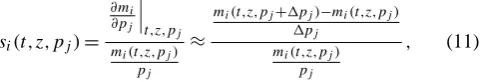
si(t,z,pj)= ∂mi ∂pj t,z,p
j mi(t,z,pj)
pj ≈
mi(t,z,pj+1pj)−mi(t,z,pj) 1pj
mi(t,z,pj) pj
, (11)
wheremi denotes measured quantityi(e.g. the water flux at
the upper boundaryjw) andpjis the value of thejth
param-eter. si is a dimensionless quantity normalised by the
mea-sured quantity and parameter value which allows to compare the sensitivities of different measured quantities and different parameters, and is (except for numeric noise caused by the numeric differentiation) independent of the step size1pj. It
is a measure how much the quantityichanges when chang-ing parameterj. Whensij is positive, quantityi increases
when increasing parameterj, when it is negative, quantity
idecreases. The larger the absolute value ofsij, the higher
[image:4.595.78.257.284.385.2] [image:4.595.308.550.526.567.2]encountering a zero crossing ofsij, quantityichanges in
op-posite directions before and after the crossing, while it is not affected by parameter changes directly at the zero point. The results of the sensitivity analysis were used to optimise the boundary conditions of the experiment.
To check whether the data measured in the experiment is sufficient to identify a unique set of soil hydraulic parame-ters, response surfaces were calculated for all scenarios (sim-ilar to Toorman et al. (1992) for the onestep outflow experi-ment and ˇSim˚unek et al. (1998) for traditional evaporation experiments). Two parameters were varied independently while all other parameters were kept at their true values. The
χ2surface, defined by Eq. (9), is then displayed in contour plots. The true value of two parametersj andkwere mul-tiplied by factorsγj andγk,pj,test=γjpj,true. The factors γ were varied from 0.1 to 2 in steps of 0.1 and from 2.2 to 3.8 in steps of 0.4, respectively. Theχ2value corresponding to a certain parameter combination was then colour-coded in a(γj,γk)plot. If one localised minimum with spherical
isolines exists in the contour plot this indicates a well posed problem. Valleys in theχ2surface indicate correlations be-tween parameters, sinceχ2stays relatively constant although two parameters were changed. This makes it more diffi-cult to identify a unique set of parameters. Multiple minima would indicate a non-unique solution. While this approach only shows a subset of the true five-dimensional parameter space along parameter planes and new features might occur in the intermediate space, it is nevertheless a good indicator whether one unique and identifiable minimum exists. Re-sponse surfaces were also used to investigate if adding more observables yields substantially more information for the in-version process.
Finally, it was checked how well the inverse model con-verges to the real parameters given the measurement error and the cross correlation between the model parameters. The forward model was used to generate synthetic data for the best combination of observations as determined from the re-sponse surfaces. Random noise normally distributed with a standard deviation ofσi was added to the data, whereσi is
the measurement uncertainty in the evaporation experiment (Table 3) as determined in Schneider et al. (2006). Five dif-ferent data sets were generated for each scenario to account for the random influence of measurement noise. From each of this data sets, the parametersα,n,Ks andθs of the van Genuchten/Mualem model and the resistance of the bound-ary layer rb were estimated with a variety of initial condi-tions. 10 parameter sets were randomly created in the range reasonable for the soil under examination. A logarithmic ran-dom distribution between the upper and the lower limit was used. These sets were used as start parameters for the gradi-ent based inversion process resulting in 50 sets of estimated parameters for each soil. This approach combines a Monte-Carlo method with the Levenberg-Marquardt minimisation. We call this a Monte-Carlo Levenberg-Marquardt method, MCLM. The inverse solutions were then compared with the
w
regime II
regime I
potential in 2cm 1
2 boundary condition
/ kPa
p
outflux −1e0
−1e1
−1e2
potential / kPa
−1e3
−1e4
−1e5 500 400 300 200
time / h 100
0 0 0.05 0.1
outflux / (mm/h)
[image:5.595.310.544.63.240.2]0.15 0.2 0.25
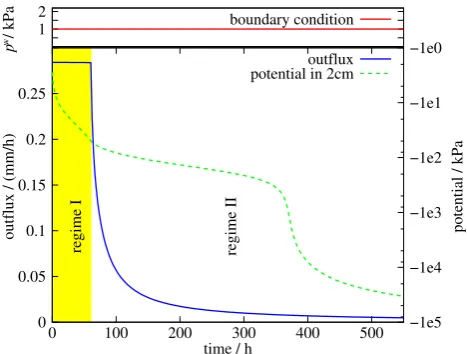
Fig. 2. Water flux at the upper boundaryjwand potential in 2 cm depth of the onestep measurement. Notice thatpwjumps from equi-librium to 1 kPa att=0.
real parameters and the resulting hydraulic functions with the true functions. A deviation coefficient was defined according to
d:=pinv−ptrue ptrue
(12) wherepinvdenotes the inverted andptruethe true parameter.
3 Results
As the results are quite similar for the three different soil types, we discuss only the results for the silt in detail. The results of the inverse modelling are given for all three soil types.
3.1 Onestep experiment
3.1.1 Physics of the process
The most simple scenario for an evaporation experiment which is also used in classical evaporation experiments is a onestep experiment as shown in Fig. 2. After saturation the sample is exposed to a constant vapour pressure at the upper boundary resulting in a progressive drying of the sample.
t t t
b.c. matric potential
sample depth
1 2 3
boundary layer
conductivity boundary layer
sample depth
t t
3
t2
[image:6.595.117.487.65.203.2]1
Fig. 3. Sketch of the potential (left) and conductivity (right) development in regime I.
(a)
1 2 3 4
5
6
−1e5 −1e4 −1e3 −1e2 −1e1 −1e0 109
8 7 6 5 4 3 2 1.5 1 0.5 0.25 0.1 0.01 0
sample depth / cm
potential / kPa t = 1.0h t = 35.4h t = 60.1h t = 62.0h t = 139.5h t = 550.9h b.c.
(b)
6 5 4
3 2 1
0.01
0.1
0.25
0.5
sample depth / cm
1
1.5 2
3
4 5 6 7 8 9
0 0.05 0.1
water content 0.15 0.2 0.25 0.3 t = 1.0h t = 35.4h t = 60.1h t = 62.0h t = 139.5h t = 550.9h
(c)
6 5
4 3 2 1
0.1
0.25
0.5
1
1.5 2
3 4 5 6 7 8 9
1e−20 1e−16 1e−12 1e−8 1e−4 1e0
conductivity / (cm/h) t = 1.0h
t = 35.4h t = 60.1h t = 62.0h t = 139.5h t = 550.9h 0.01
sample depth / cm
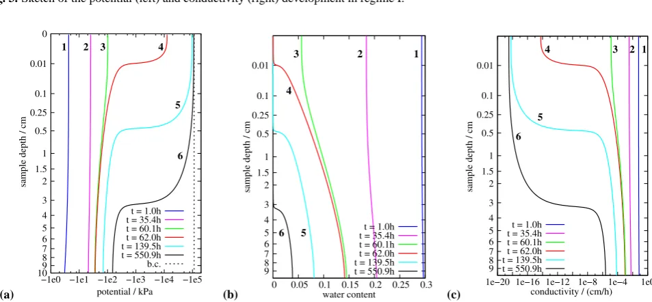
Fig. 4. Potentialψm(z)(a), water contentθ`(z)(b) and hydraulic conductivityK(θ (z))(c) distributions for the onestep experiment at different timesti: (1) at an early time in regime I, (3) directly before the transition to regime II, (4) a short time later after the transition, (6) at the end of the experiment. Notice the non-linear scaling of the depth axis.
near the surface for three times is shown in Fig. 3. The ma-jor part of the potential drop is caused by the resistance of the boundary layer. Due to the much higher conductivity in the soil, water is delivered to the evaporating surface with a minimal gradient, which can also be seen in the simulation results (Fig. 4a). Hence, the hydraulic properties have only a minimal influence on the flux. However, the potential of the sample changes with time due to the successive drying of the soil. Measurements of potential could therefore give in-formation about the hydraulic properties of the sample. For
t.20 h, the potential in the soil is above−10 kPa and there-fore can be measured easily with a tensiometer. However, due to the small deviations from the linear decrease (which would be expected for a hydraulic conductivity which is con-stant over the whole sample), one would need a very high accuracy to obtain information about the hydraulic conduc-tivity. As the relative permeability of the silt decreases only
slowly with decreasing water potential, a small potential gra-dient is sufficient to sustain the water flux to the soil surface and the sample dries more or less uniform over the whole whole 10 cm high sample.
With continuing evaporation the potential and the water content decrease (Fig. 4), most rapidly near the surface. Eventually the conductivity of the soil becomes limiting. Shokri et al. (2009) found at this point in their experiments the formation of a dry surface layer, which is in excellent agreement with our simulations. The system enters regime II and jw starts to decrease rapidly. This transition is quite abrupt because (i) the functionK(θ`)is very steep in the
[image:6.595.57.534.220.441.2]unsaturated and dry zone with very steep gradients) forms at the surface and then moves into the soil (Fig. 4). Since the low-conductive layer (the distance inside the soil to be passed by vapour diffusion) grows with continuing evaporation, the flux continues to decrease.
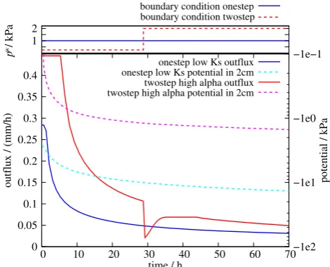
Regime I occurs only if the saturated hydraulic resis-tance (the reciprocal of the saturated hydraulic conductiv-ity), which is the lowest possible resistance inside the soil, is lower than the resistance of the boundary layer. This is illustrated by reducing Ks by a factor of 20, resulting in
Ks=0.05 cm/h (Fig. 5, blue and dashed cyan curves).Ksis now lower than the flux which can be evaporated through the soil-atmosphere boundary layer. Thus, the sample directly enters regime II.
3.1.2 Sensitivity analysis
The relative sensitivity coefficients according to Eq. (11) were calculated for each measurement type for all hydraulic parameters (Fig. 6).
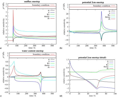
As the system is in regime I at the start of the experi-ment, the water flux is limited by the resistance of the soil-atmosphere boundary layer alone. At early times, the outflux
jwis therefore most sensitive torbwhile the sensitivity to all other parameters is very small.
When the topmost layer of the soil has dried out, the soil hydraulic properties, in particular the hydraulic conductiv-ity, become limiting for the evaporation rate. The evapora-tion flux is most sensitive to all parameters exactly at the bend point where the system enters regime II and the out-flow starts to decrease after the plateau. The sensitivity on
rbdecreases continuously because the drier the sample, the less important is the resistance of the boundary layer. Asθs scales the amount of available water whenθris held constant, the sensitivity ofθs stays more or less constant after a quick decay. For all other parameters the sensitivity decreases after the maximum and after a zero-crossing eventually increases again with opposite sign. The zero-crossing can be explained by mass conservation. As the total water content of the sam-ple is constant, a higher evaporation at earlier times has to be compensated by lower evaporation towards the end of the experiment and vice versa.
In contrast to the evaporation flux, the potentialψm is at the beginning of the experiment most sensitive toα andn
which control the shape of the soil water retention curve.Ks is the only parameter for which the sensitivity is nearly zero during regime I. The sensitivity onrbandθs are less impor-tant at the beginning, but increase during regime I and reach a maximum at the transition to regime II as well as the sensi-tivity onn.
Sincerbdetermines the speed of drainage in regime I, it is clear that the potential, which is connected to the water con-tent by the water characteristic, is also dependent onrb. This effect will become more pronounced as time passes because the longer a different outflux caused by a differentrbis
re-w
−1e−1
−1e0
potential / kPa
−1e1
−1e2 70 60 50 40 time / h 30 20 10 0 0 0.05 0.1 0.15
outflux / (mm/h)
0.2 0.25 0.3 0.35 0.4
/ kPa
p
2 1
onestep low Ks outflux onestep low Ks potential in 2cm boundary condition onestep boundary condition twostep
[image:7.595.309.544.64.254.2]twostep high alpha outflux twostep high alpha potential in 2cm
Fig. 5. Water flux at the upper boundaryjwand potential in 2 cm depth for the “onestep” experiment with 20 times lowerKs, as well as for the twostep experiment with 20 times higherα. The former stays virtually no time in regime I due to the very low conductivity. The latter shows a more distinct switch-back to regime I but struc-turally it is identical to the original soil. Notice thatpwjumps from equilibrium to 1 kPa and 0.25 kPa, respectively, att=0.
tained, the higher are also the differences in the potential.θs determines the amount of available water. With a constant evaporation rate, the more water is available, the less is the relative change of water content and therefore the change of potential when all other parameters are kept constant. Thus, the behaviour ofθsis analogous to the one ofrb.
The maxima are much less pronounced than for the evap-oration flux. For all parameters the sensitivity is more or less constant or increases slowly in regime II and reaches a large peak att≈370 h which is caused by the passing of the dry-ing front at the tensiometer position. This peak is discussed in more detail in Sect. 3.2.2. A zero-crossing only exists for
nas onlyninfluences the shape of the soil water retention curve. The generally higher sensitivity in the dry range is in accordance with the result of ˇSim˚unek et al. (1998) for tra-ditional evaporation experiments. As they pointed out, the water characteristic becomes steeper for more negative po-tentials and thus parameter changes have more influence at lower potentials.
(a)
w
outflux onestep
500 400
300 time / h 200 100
0 −2 −1 0 relative sensitivity 1 2 3 4 5 6 7
p
/ kPa
α
n Ks thetas rb 1
2
boundary condition
(b) w 1
2
boundary condition
/ kPa
p
relative sensitivity
20
15
10
5
0
−5
−10
−15
0 100 200
time / h
300 400 500
potential 2cm onestep
rb
thetasKs
n α
(c)
w 1
2 boundary condition
0.8
0.6
0.4
0.2
relative sensitivity
0
−0.2
−0.4
−0.6
−0.8
0 100 200
time / h
300 400 500
water content onestep
/ kPa
p
rb
thetasKs
n
α
(d)
α
potential 2cm onestep (detail)
n Ks thetas rb
100 80
60 time / h 40 20
0 −2.5
−2 −1.5 −1 −0.5
relative sensitivity
[image:8.595.56.547.63.470.2]0 0.5 1 1.5
Fig. 6. Sensitivity coefficientss(t )for the onestep experiment for the outflux (a), the potential in 2 cm (b) and the water content in 2 cm (c). A detail view of the first 100 h for the potential in 2 cm is shown in (d). Notice thatpwjumps from equilibrium to 1 kPa att=0.
The sensitivity to changes of the saturated hydraulic con-ductivity is rather low for all types of measurements and reaches significant values only for the evaporation at the tran-sition point and at the passing of the drying front.
3.2 Multistep experiments
3.2.1 Physics of the process
As the transition from regime I to regime II contains much information, one would suggest that multistep experiments can drastically improve the sensitivity if it is possible to re-produce the switch from regime I to regime II with boundary condition steps. To switch from regime II back to I, either the conductivity in the upper soil or the resistance of the bound-ary layer must be increased, or the potential drop on the boundary layer decreased. As the resistance of the boundary
layerrbis constant, this cannot be achieved by lowering the boundary potential. Lowering the boundary potential speeds up the drainage of the sample but does not lead to new fea-tures.
(a)
1 4 3 2 0
0.01
0.1
0.25
0.5
1
1.5 2
3
4 5 6 7 8 9
−1e1 −1e3 −1e5
−1e−1
potential / kPa
sample depth / cm
t = 28.7h t = 34.2h t = 46.0h t = 550.3h b. c. t = 28.7h b. c. t = 34.2h, 46.0h, 550.3h
(b)
2
3
1
4
0.01
0.1
0.25
0.5
1
1.5 2
3
4 5 6 7 8 9
0 0.05 0.1
water content 0.15 0.2 0.25 0.3 t = 28.7h
sample depth / cm
t = 34.2h t = 46.0h t = 550.3h
(c)
2 3 4
1 0.01
0.1
0.25
0.5
1
1.5 2
3
4 5 6 7 8 9
1e−25 1e−20 1e−15 1e−10 1e−5 1e0
conductivity / (cm/h)
sample depth / cm
[image:9.595.64.536.63.258.2]t = 28.7h t = 34.2h t = 46.0h t = 550.3h
Fig. 7. Potentialψm(z)(a), water contentθ (z)(b) and hydraulic conductivityK(θ (z))(c) distributions for the twostep experiment with 20
times higherα: (1) directly before the first boundary condition switch, (2) after relaxation, (3) after re-entering regime II and (4) at the end of the experiment. Notice the non-linear scaling of the depth axis.
potential at the soil surface, resulting in a larger potential drop on the boundary layer and therefore an again higher evaporation flux (see Fig. 7). When this adaptation stage is finished, the increase of water content in the upper soil and therefore the increase of the evaporation rate ends, the deliv-ery from below and the evaporation flux are equal again. If the change in the boundary condition was large enough, the resulting evaporation flux at this point is low enough to be sustained by the soil for a longer time span and regime I is reached again, else the system stays in regime II. This de-pends on the relation between the new potential drop on the boundary layer and the hydraulic conductivity in the soil (soil water state).
The same effect also occurs with the normal value ofα, but it is harder to see (after the first boundary condition jump att=62.5 h in Fig. 8 red line). The higherαresults in a less negative potential in the soil before the switch and a relax-ation to a higher water content after the switch. Therefore it takes longer until the conductivity drops low enough to reach regime II again.
We acknowledge that any change in the direction of flow leads to hysteresis, which was not considered in the simula-tion. However, hysteresis is most pronounced in coarse tex-tured porous media and in the wet range of experiments. In our numerical multistep experiments, the switch occurs only in the dry range where water vapour is the only relevant trans-port mechanism. Thus hysteresis should be negligible.
The twostep experiment has the disadvantage that the po-tential range covered is too small during a reasonable mea-suring time. This can be compensated by applying a third step after the experiment has entered the hydraulically dom-inated regime again to speed up drainage. This results in a threestep experiment (Fig. 8, red and dashed magenta
w
outflux −1e0
−1e1
−1e2
−1e3
−1e4
−1e5 500 400 time / h
300 200 100 0
0 0.05 0.1 0.15 0.2 0.25 0.3 0.35 0.4 1
2 boundary condition
/ kPa
p
outflux / (mm/h) potential / kPa
potential in 2cm, no vapour transportoutflux, no vapour transport
potential in 2cm
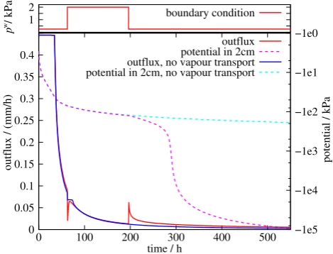
Fig. 8. Influence of water vapour transport on the results: The three-step experiment was simulated taking vapour transport inside the soil into account (the normal case, red) and without considering it (blue). Notice thatpwjumps from equilibrium to 0.25 kPa att=0. For more explanations see Sect. 3.2.1.
curves) which has identical general features as the twostep experiment but has a much larger potential range in 2 cm depth during the same measuring time.
[image:9.595.309.544.328.507.2]w 1
2 boundary condition
outflux threestep2
α
500 400 300 time / h 200 100 0 −2
0 2
relative sensitivity
4 6 8
p
/ kPa
rb thetasKs n
w 1
2 boundary condition
30
20
relative sensitivity
10
0
−10
−20
−30
0 100 200 300 400 500
time / h
potential 2cm threestep2
/ kPa
p
α
n Ks thetas rb
w 1
2 boundary condition
0.6 0.4 0.2
relative sensitivity
0 −0.2 −0.4 −0.6 −0.8 −1
0 100 200 300
time / h 400 500
α
water content threestep2
/ kPa
p
[image:10.595.73.523.64.189.2]n Ks thetas rb
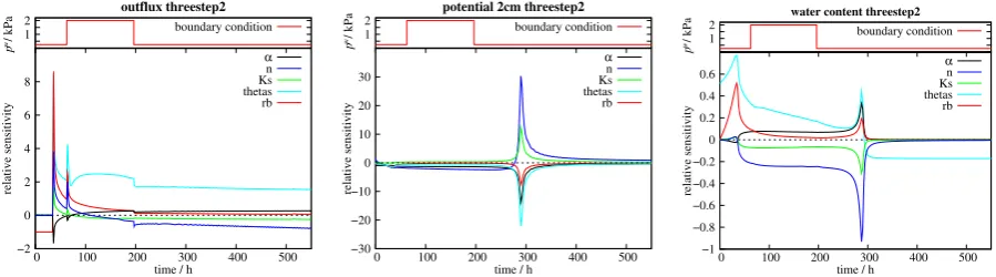
Fig. 9. Sensitivity coefficientss(t )for the threestep experiment for the outflux (left), the potential in 2 cm (middle) and the water content in 2 cm (right). Notice thatpwjumps from equilibrium to 0.25 kPa att=0.
about the soil hydraulic properties is required to choose the optimal boundary condition steps in a multistep experiment. This knowledge could be obtained by first performing a on-estep experiment and then using this information to design a multistep experiment. However, a major disadvantage of this scheme is the long time required to conduct two experi-ments.
To study the importance of water vapour flow inside the soil compared to the flow of liquid water, we also performed a simulation where the effective conductivity contributed by water vapour flow was disabled (Fig. 8). Water vapour flow inside the soil is especially important at later times, when the soil becomes very dry after the third step of the boundary condition att=196.3 h. Without the water vapour transport the hydraulic conductivity is already too low to get an in-crease of the evaporation flux when the vapour pressure at the boundary is reduced. The sample is effectively sealed by a very dry layer at the sample surface with very low conduc-tivity, which prevents the further drying of deeper regions. A second feature not present in the simulation without vapour transport in the soil is the “undershoot” of the evaporation at the transition back to boundary layer dominated regime at
t=62.5 h. With vapour transport, the evaporation before the switch is higher and thus the potential at the surface is lower. This results in a more pronounced drop of the evaporation and a longer time till the dynamic equilibrium in the soil is reached again.
3.2.2 Sensitivity analysis
While there is no big change in the relative sensitivities for the potential and the water content 2 cm below the soil sur-face compared to the onestep experiment, the sensitivities of jw increase substantially for experiments that re-enter regime I (Fig. 9). Multistep experiments which do not re-enter regime I show no strong effect in the sensitivities (data not shown here). Thus, multistep experiments are a good tool to increase the sensitivity. Considering the larger poten-tial range which is covered by the threestep experiment, it is
also considered superior to the corresponding twostep exper-iment.
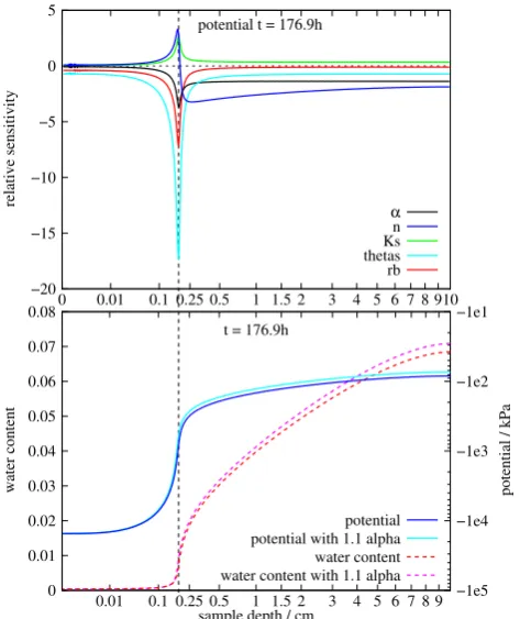
To determine the optimal position of a tensiometer or per-mittivity probe, profiles of relative sensitivity have been anal-ysed. Figure 10 (top) shows profiles of the relative sensitivity of the matric potential to changes inα. Generally, the sen-sitivity is lower near the sample surface especially at later times. After the onset of regime II, a large sensitivity peak appears, which moves downward with time. Att=44 h the sensitivity drop below the peak even leads to a zero-crossing of the sensitivity. After the increase of water vapour pressure at the upper boundary and the transition back to regime I the sensitivity peak vanishes for a short time and reappears after the fall-back to regime II. This is the result of a rewetting of the top soil, which is caused by the fluxes from below which are higher than the (reduced) evaporation rate.
The peaks are located at the drying front (as can be seen fort=176.9 h from a comparison with Fig. 11) where the gra-dients are particularly high and thus small deviations in the parameters lead to large changes in the solution. As changes of the parameters also affect the position of the drying front, small parameter changes generate huge potential differences in its proximity. Figure 11 illustrates the change in the pro-files of matric potential and water content att=176.9 h ifαis increased by 10%. A zero-crossing of the sensitivity occurs if the parameter change leads not only to a different position, but also to a change in the steepness of the drying front.
This is in accordance to Romano and Santini (1999) who reported that sensitivities of the matric potential in traditional evaporation experiments in the uppermost part of the soil show increasing curvatures and a drop to zero. They no-ticed that this especially happens at larger times when “1h
changes its sign in close proximity to the evaporating sur-face”, where1his the change of matric head. A change in the sign of1h corresponds to a change of the sign of the corresponding sensitivity coefficient as it was found in our study.
50 5
relative sensitivity
3
1
−1
−3
−5
0 0.01 0.1 0.25 0.5 1 1.5 2 3 4 5 6 78910 potential alpha
sample depth / cm
t = 9.2h t = 44.0h t = 74.5h t = 176.9h t = 388.2h
water content alpha 5
3
1
−1
−3
−5 −50
relative sensitivity
0 0.01 0.1 0.25 0.5 1 1.5 2 3 4 5 6 7 8 910
sample depth / cm
t = 9.2h t = 44.0h
t = 176.9ht = 74.5h
[image:11.595.310.547.63.345.2]t = 388.2h
Fig. 10. Relative sensitivitys(z,ti)onαof the potentialψm(top) and the water contentθ(bottom), respectively, versus heightzfor different timesti, both for the threestep experiment. Note the switch in the sensitivity scale, marked with a dashed black line, and the non-linear scaling of the depth axis.
sensitivity at the soil surface and a zero-crossing which is located above the peak at the drying front for later times.
In principle the profiles of the relative sensitivity are sim-ilar for all parameters. As shown in Fig. 11 the profiles of the sensitivity of the matrix potential att=176.9 h for differ-ent parameters mainly differ in the size and the sign of the peak. The sensitivity to changes ofnhas a very pronounced zero-crossing asnalways influences the steepness of the dry-ing front. The sensitivity peaks are most pronounced for the parametersθs andrbas these parameters have the strongest influence on the propagation speed of the drying front, by determining the speed of drainage in regime I and thus the starting time of the drying front movement.
For the permittivity probe a position nearer to the surface than the 2 cm we used would be advantageous as the sensitiv-ity of the water content is always high there, but this is hard to realise experimentally. For the tensiometer a depth of 2 cm is quite fine, as the sensitivity at this depth is high except for very late times after the passing of the drying front. When
0.01 0.1 0.25 0.5 1 1.5 2 3 4 5 6 7 8 910 −20
−15 −10 −5 0 5
0 0.01 0.02 0.03 0.04 0.05 0.06 0.07 0.08
9 8 7 6 5 4 3 2 1.5 1 0.5 0.25 0.1 0.01
−1e1
−1e2
−1e3
−1e4
−1e5
sample depth / cm
potential / kPa
water content
0
relative sensitivity
t = 176.9h potential t = 176.9h
Ks thetas
α
n
rb
potential potential with 1.1 alpha water content water content with 1.1 alpha
Fig. 11. Relative sensitivitys(z,t )of the potentialψmon all vari-ables at t=176.9 h (top). The potential and water content pro-files for the undisturbed parameters as well as withαchanged by 10 % (bottom) illustrate the source of the huge sensitivity peaks at
z≈0.15 cm in the plot above, the location is marked with a dotted vertical line. Note the non-linear scaling of the depth axis.
the drying front passes, the potential drops so low (−104kPa – this corresponds to −1 km water column – or less, see Fig. 11, bottom) that it is outside the measurement range of traditional tensiometers. Thus, for a real measurement ten-siometers have to be removed before the drying front passes to avoid a leakage of water into the soil and therefore the sen-sitivity peaks of potential cannot be utilised with traditional tensiometers.
[image:11.595.51.283.64.389.2]n/ n0
1 2 3
1 2 3
Ks
/K
s,
0
1 2 3
1 2 3
θs
/θ
s,
0
1 2 3
1 2 3
rb
/
rb,
0
1 2 3
1 2 3
α/α0 α/α0 α/α0 α/α0
Ks
/K
s,
0
1 2 3
1 2 3
θs /θs,
0
1 2 3
1 2 3
rb
/
rb,
0
1 2 3
1 2 3
θs /θs,
0
1 2 3
1 2 3
n/n0 n/n0 n/n0 Ks/Ks,0
rb
/
rb,0
1 2 3
1 2 3
rb
/
rb,0
1 2 3
1 2 3
χ
2
100.0 6.1e+2 3.8e+3 2.3e+4 1.4e+5 8.6e+5 5.3e+6
[image:12.595.133.464.62.306.2]Ks/Ks,0 θs/θs,0
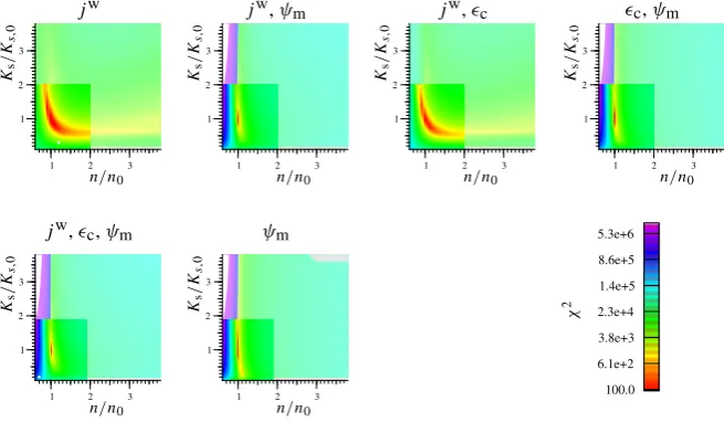
Fig. 12. Response surfaces for the threestep experiment withjwandψmas target variables. The light regions with deviation coefficients
larger than 2 were calculated with a smaller resolution of 0.4. Non-matching structures between the two regions are caused by the different resolution. Note that aχ2above 107is displayed in white, points where the model did not finish after 120 000 time steps is marked grey.
jw jw,ψm jw,c c,ψm
Ks
/K
s,
0
1 2 3
1 2 3
Ks
/K
s,
0
1 2 3
1 2 3
Ks
/K
s,
0
1 2 3
1 2 3
Ks
/K
s,
0
1 2 3
1 2 3
n/n0 n/n0 n/n0 n/n0
jw,c,ψm ψm
Ks
/K
s,
0
1 2 3
1 2 3
Ks
/K
s,
0
1 2 3
1 2 3
χ
2
100.0 6.1e+2 3.8e+3 2.3e+4 1.4e+5 8.6e+5 5.3e+6
[image:12.595.133.461.367.558.2]n/n0 n/n0
Fig. 13. Same as Fig. 12 but with different target variable combinations. Note that real permittivity measurements have large errors in the dry range, which would lead to much worse results for the casec+ψm.
3.3 Response surfaces
Figure 12 shows the response surfaces of the threestep exper-iment withjw andψm as target variables. The tensiometer was removed at−30 kPa. Generally, there is a single global minimum and it is relatively well-defined. Only the com-binations(α,Ks),(n,Ks),(Ks,θs), and(Ks,rb)whereKsis involved have small valleys and the slope to the absolute min-imum in the direction of the valleys is low. This is a
K. Schneider-Zapp et al.: Numerical analysis of evaporation experiment 777
22 K. Schneider-Zapp et al.: Numerical analysis of evaporation experiment
−30kPa −70kPa
n/n
0
1 2 3
1 2 3
n/n
0
1 2 3
1 2 3 χ 2 100.0 6.1e+2 3.8e+3 2.3e+4 1.4e+5 8.6e+5 5.3e+6
[image:13.595.318.534.60.471.2]α/α0 α/α0
Fig. 14.Same as Fig. 12 but for different tensiometer tear-off valuesψlimitwithjwandψmas target variables.
−
30
kPa
−
70
kPa
n/n
0
1 2 3
1 2 3
n/n
0
1 2 3
1 2 3 χ 2 100.0 6.1e+2 3.8e+3 2.3e+4 1.4e+5 8.6e+5 5.3e+6
α/α0 α/α0
Fig. 14.
Same as Fig. 12 but for different tensiometer tear-off values
ψ
limitwith
j
wand
ψ
mas target variables.
Fig. 14. Same as Fig. 12 but for different tensiometer tear-off values ψlimitwithjwandψmas target variables.
To identify the essential measurements for a good estima-tion of the parameters the response surfaces of the threestep experiment forKs andnfor combinations of the three mea-surement types are analysed (Fig. 13) asKsis especially hard to estimate due to its low overall sensitivity. If only the evap-oration fluxjwis used the residual does not have a well de-fined minimum but more a banana like shaped extended re-gion. The minimum in the direction ofnis better defined if only the matric potential in 2 cm depth is used but there is still a very long valley in the direction ofKs. This valley becomes much shorter if a combination ofjw andψm is used. The addition of permittivity (i. e. water content) measurements improves the situation only in the combination c+ψm, in all cases involving the evaporation flux the changes are very small. However, it should be noted that accurate permittivity measurements (e.g. with TDR probes) in the dry range are not feasible. The reasons are: (i) Since the traveltime error is constant, the relative error increases with decreasingc. (ii) The compound permittivitycis a function of the soil matrix permittivitys, of the porosityφ, and the actual geometry. For low water contents, the uncertainty of the measurement diverges since the permittivity contribution of the remaining water becomes equal to or even lower thans,φis not known accurately, and the geometry is unknown. (iii) For thin films of water as found in the dry region,w is different from the one of bulk water. Additionally, the measurement volume which was neglected in the simulations will smear out gra-dients, and results are expected to be worse than in the ideal case of a point measurement.
Asjwis the derivative of the total water content, it is rea-sonable that adding a water content measurement does only give slightly more information. In contrast, ψm is an in-dependent observable and therefore gives more information about the soil water retention curve. However the fundamen-tal difficulties with tensiometers must be regarded. The in-formation is only provided in a small potential window and great care must be taken that the tensiometer is removed be-fore the potential in the soil drops below its air entry point, or the water vapour pressure, whatever is higher. Therefore it was also investigated whether a tensiometer which can mea-sure up toψm=−70 kPa or even without a limit makes a
con-(a) 0 0.05 0.1 0.15 0.2 0.25 0.3 0.35 0.4 0.45 0.5
0 100 200 300 400 500 −30
−25 −20 −15 −10 −5 0
flux / (mm/h) potential / kPa
time / h
model flux rejected
rawdata flux model potential rejected
rawdata potential model potential accepted model flux accepted
rawdata potential rawdata flux
(b) 0
−0.5 −1 −1.5 −2 −2.5 −3 −3.5 200 180 160 140 120 100 80 60 40 20 0 0 0.1 0.2 0.3 0.4 0.5 0.6 0.7 0.8 0.9 1
flux / (mm/h)
time / h
potential / kPa
model potential acceptedmodel potential rejected model flux acceptedmodel flux rejected
(c) 0 0.1 0.2 0.3 0.4 0.5 0.6
0 100 200 300 400 500 −30
−25 −20 −15 −10 −5 0
flux / (mm/h) potential / kPa
time / h
model flux rejected
rawdata flux model potential rejected
rawdata potential model flux accepted
model potential accepted
Fig. 15. Comparison between the accepted fits with the largest residuum and the rejected fits with the lowest residuum, for sand (a) (residuum 4900 (accepted) vs. 9700 (rejected)), loamy sand (b) (residuum 28 000 vs. 3300), and silt (c) (residuum 4600 vs. 7300), respectively. The reason for rejecting the curves were for (a) the deviation of the tensiometer, for (b) the first plateau was not repre-sented, and for (c) the first peak was not reprerepre-sented, respectively. Note that for (b), although the potential of the accepted fit matches worse than in the accepted one, its deviation is just at the sort-out limit and limit cases were still accepted, while the plateau in the rejected fit is definitely not represented at all.
[image:13.595.54.288.71.166.2]0 0.1 0.2 0.3 0.4 0.5 0.6 0.7 0.8 0.9 1
-1e0 -1e1
saturation
potential / kPa 38 of 42 fits overlapping
1e-10 1e-8 1e-6 1e-4 1e-2 1e0 1e2
0 0.2
0.4 0.6
0.8 1
conductivity / (cm/h)
saturation
0 0.1 0.2 0.3 0.4 0.5 0.6 0.7 0.8 0.9 1
-1e-1 -1e0
-1e1 -1e2
-1e3
saturation
potential / kPa 12 of 27 fits overlapping
1e-12 1e-10 1e-8 1e-6 1e-4 1e-2 1e0
0 0.2
0.4 0.6
0.8 1
conductivity / (cm/h)
saturation
0 0.1 0.2 0.3 0.4 0.5 0.6 0.7 0.8 0.9 1
-1e0 -1e1
-1e2 -1e3
-1e4
saturation
potential / kPa 32 of 34 fits overlapping
1e-14 1e-12 1e-10 1e-8 1e-6 1e-4 1e-2 1e0
0 0.2
0.4 0.6
0.8 1
conductivity / (cm/h)
[image:14.595.52.546.62.510.2]saturation
Fig. 16. Hydraulic functions of the inverse solutions (grey), and the functions for the true parameters (black line), for the sand (top, 42 fits, 38 practically overlapping), sandy loam (middle, 27 fits, 12 practically overlapping), and silt (bottom, 34 fits, 2 deviating slightly), respectively.
tensiometers with a much wider range of measurements like the ones presented by Bakker et al. (2007) would be most helpful for this type of experiment.
3.4 Convergence study
The convergence study revealed the existence of local min-ima which are not visible in the response surfaces, because they are not located in two-dimensional sub-planes of the five-dimensional parameter space. When initially running the inverse fits with potential and outflux data, the conver-gence was poor. The reason was that when the outflux peaks did not fit initially and the algorithm slightly modified the
Table 4. Results of the convergence study withjwandψmas target variables. For the resulting parameters and standard deviations from the model output, as well as the deviation coefficientsddefined by Eq. (12), mean and variance of the inversion of the start parameter sets with each of the data sets are shown.
Sand (42 fits)
parameter unit real value result standard deviation deviation coeff.d
α m−1 5 4.90±0.04 0.024±0.001 -0.020±0.009
Ks cm h−1 2 2.11±0.07 0.014±0.002 0.05±0.04
φ m3m−3 0.3 0.2985±0.0003 0.00076±0.00001 -0.0049±0.0009
rb mm 3 3.013±0.003 0.0086±0.0002 0.004±0.001 n – 4 4.2±0.1 0.0218±0.0008 0.05±0.02
Sandy loam (27 fits)
parameter unit real value result standard deviation deviation coeff.d
α m−1 10 8.6±0.5 0.045±0.005 -0.14±0.05
Ks cm h−1 0.1 0.08±0.01 0.0010±0.0001 -0.2±0.1
φ m3m−3 0.3 0.309±0.003 0.00090±0.00001 0.03±0.01
rb mm 3 2.83±0.08 0.020±0.002 -0.06±0.03 n – 2 2.18±0.07 0.0062±0.0004 0.09±0.03
Silt (34 fits)
parameter unit real value result standard deviation deviation coeff.d
α m−1 0.5 0.503±0.003 0.0012±0.0001 0.006±0.006
Ks cm h−1 0.1 0.12±0.02 0.0007±0.0002 0.2±0.2
φ m3m−3 0.3 0.298±0.003 0.00074±0.00005 -0.01±0.01
rb mm 3 3.02±0.05 0.011±0.001 0.01±0.02 n – 2 2.000±0.009 0.0052±0.0004 0.000±0.004
(this corresponds to 1 kPa), and (3) the outflux plateau at the beginning of the experiment was not reproduced at all. Fig-ure 15 shows a comparison between the accepted fit with the highest residuum and the rejected fit with the lowest residuum for all investigated soils.
Using this procedure, the parameters were reasonably re-produced. The mean and standard deviation of the estimated values for each parameter is given in Table 4, the hydraulic functions for all converged fits together with the ones for the true parameters are shown in Fig. 16. The deviations in each column of Table 4 were calculated from the ensemble mean of converged results. When comparing the results of the in-version and its standard deviation calculated from the analy-sis of the sensitivity matrix with the real parameters and the variance encountered by the different fits in the ensemble, one can see that the standard deviations calculated from the analysis of the sensitivity matrix are too small in almost all cases. This is attributed to the fact that the sensitivity ma-trix does only give a linear approximation of the uncertain-ties. Deviations of the resulting fit parameters are quantified by the deviation coefficientd. No systematic deviations are found for the silt, however small systematic deviations are present for the sand and the sandy loam. This is expected, since the evaporation method is most sensitive in the dry range, where dynamics of the silt actually take place, but it
is relatively insensitive for the wet range, the region of most of the dynamics of the sand and sandy loam soil. The silt has the smallest deviations since its dynamics are reaching most into the dry region of the three soils. This is also confirmed by the plots. For the water characteristic of the sand with 42 fits, 38 practically overlap while 4 deviate quite a bit. The sandy loam has the most significant deviations of all three soils in the water characteristic, only 12 of 27 fits are prac-tically overlapping and 3 have small deviations, while the remaining 12 fits are relatively bad. The silt is nicely rep-resented in all fits, only 2 of 34 fits are deviating slightly. Considering that the estimation of the hydraulic conductiv-ity is difficult, the conductivconductiv-ity function is well represented for all soils. The analysis shows that applying the Monte-Carlo Levenberg-Marquardt approach for real experimental data would lead to a reasonable estimate of the parameters, since most fits converge to the correct parameters and the few deviating fits could be identified in the ensemble.
4 Conclusions
outflux is limited by the diffusive soil-atmosphere boundary layer, while in regime II it is limited by the hydraulic prop-erties. The sensitivity analysis showed that the sensitivity is especially high at the transition between the two regimes. In regime II, a drying front penetrates through the soil. At the location of this front, sensitivity is very high but this sen-sitivity peak can only partially be exploited as the potential drops below the measurement range of traditional tensiome-ters. However, if a profile measurement of water content is available the sensitivity peak allows to scan different layers of the sample. Positioning the tensiometer and the permittiv-ity probe 2 cm below the sample surface gives a good sensi-tivity over the whole experiment.
As the transitions between these two regimes can be in-duced by boundary condition changes, a threestep experi-ment, where the water vapour pressure at the boundary is temporarily increased after regime II was reached, yields an increased sensitivity and a high measurement range.
The analysis of the response surfaces exhibited a single minimum for all parameters, which was mostly well lo-calised. The estimation of the saturated hydraulic conduc-tivity was improved significantly by adding a potential mea-surement to the outflux meamea-surement. In contrast, adding a water content measurement yields no noticeable improve-ment. However, a combination of permittivity and tensiome-ter measurements gave nearly as good a response surface as a combination of evaporation flux and tensiometer measure-ments. However TDR probes which are typically used for water content measurements are no point measurements but have a rather high sampling volume, and the uncertainty for very dry conditions diverges. Therefore it is expected that for real measurements the response surface will get much worse. Furthermore uncertainties in porosity and soil matrix permit-tivity would introduce additional errors which were not con-sidered in the simulations. Hence measuringjw will prob-ably be much more accurate in real experiments. There is a significant improvement if the measurement range of the tensiometer is extended to −70 kPa. A hypothetical ten-siometer with unlimited range shows a huge advantage. This emphasises the importance of extended-range tensiometers.
When excluding obviously diverged fits, the inverse model converged for the silt to correct solutions from all initial val-ues. For the sand and sandy loam, some fits of the ensem-ble deviated significantly while others reasonably converged to the correct parameters. The deviations were attributed to the small sensitivity of the evaporation experiment in the wet range. Usage of the Monte-Carlo Levenberg-Marquardt ap-proach allows a meaningful parameter estimation. Compar-ing the hydraulic functions estimated usCompar-ing the mean MCLM estimated parameters showed that only the water character-istic of the sandy loam deviated slightly and all others over-lapped with the true functions. The distribution of the param-eters caused by measurement errors and cross-correlation of the parameters was acceptable.
Acknowledgements. We acknowledge and greatly appreciate the constructive comments of N. Shokri, H. Fujimaki, an anonymous reviewer, and of the editor.
Edited by: W. Durner
References
Bakker, G., van der Ploeg, M. J., de Rooij, G. H., Hoogen-dam, C. W., Gooren, H. P. A., Huiskes, C., Koopal, L. K., and Kruidhof, H.: New polymer tensiometers: measuring matric pressures down the the wilting point, Vadose Zone J., 6, 196– 202, doi:10.2136/vzj2006.0110, 2007.
Foken, T.: Angewandte Meteorologie, Springer, Berlin, Heidelberg, New York, 2003.
Ippisch, O., Vogel, H.-J., and Bastian, P.: Validity limits for the van Genuchten-Mualem model and implications for parameter estimation and numerical simulation, Adv. Water Res., 29, 1780– 1789, 2006.
Jin, Y. and Jury, W. A.: Characterizing the dependence of gas dif-fusion coefficient on soil properties, Soil Sci. Soc. Am. J., 60, 66–71, 1996.
Mualem, Y.: A new model for predicting the hydraulic conductivity of unsaturated porous media, Water Resour. Res., 12, 513–522, 1976.
Murray, F. W.: On the computation of saturation vapor pressure, J. Appl. Meteorol., 6, 203–204, 1967.
Philip, J. R. and de Vries, D. A.: Moisture movement in porous ma-terials under temperature gradients, Trans. Am. Geophys. Union (EOS), 38, 222–232, 1957.
Prat, M.: Recent advances in pore-scale models for drying of porous media, Chem. Eng. J., 86, 153–164, doi:10.1016/S1385-8947(01)00283-2, 2002.
Rawlins, S. L. and Campbell, G. S.: Water potential: Thermocouple psychrometry, in: Methods of soil analysis, Part 1. Physical and mineralogical methods, edited by: Klute, A., Agronomy Series 9, 597–618, American Society of Agronomy, Madison, WI, 2nd edn., 1986.
Romano, N. and Santini, A.: Determining soil hydraulic func-tions from evaporation experiments by a parameter estimation approach: Experimental verifications and numerical studies, Wa-ter Resour. Res., 35, 3343–3359, 1999.
Roth, K., Schulin, R., Fl¨uhler, H., and Attinger, W.: Calibration of Time Domain Reflectometry for Water Content Measurement Using a Composite Dielectric Approach, Water Resour. Res., 26, 2267–2273, 1990.
Scherer, G. W.: Theory of drying, J. Am. Ceram. Soc., 73, 3–14, doi:10.1111/j.1151-2916.1990.tb05082.x, 1990.
Schneider, K., Ippisch, O., and Roth, K.: Novel evaporation exper-iment to determine soil hydraulic properties, Hydrol. Earth Syst. Sci., 10, 817–827, 2006,
http://www.hydrol-earth-syst-sci.net/10/817/2006/.
Sherwood, T. K.: The drying of solids – III Mechanism of the drying of pulp and paper, Ind. Eng. Chem., 22, 132–136, doi:10.1021/ie50242a009, 1930.
Shokri, N., Lehmann, P., and Or, D.: Critical evaluation of enhancement factors for vapor transport through unsat-urated porous media, Water Resour. Res., 45, W10433, doi:10.1029/2009WR007769, 2009.
ˇSim˚unek, J., Wendroth, O., and van Genuchten, M. T.: Parame-ter estimation analysis of the evaporation method for deParame-termin- determin-ing soil hydraulic properties, Soil Sci. Soc. Am. J., 62, 894–905, 1998.
Toorman, A. F., Wierenga, P. J., and Hills, R. G.: Parameter estima-tion of hydraulic properties from one-step out flow data, Water Resour. Res., 28, 3021–3028, 1992.