Optimization of Operating Parameters on a Diesel Engine using Grey Relational Analysis

(1)

Optimization of Operating Parameters on a Diesel Engine Using Grey

Relational Analysis

Geetha.N.K

1

_{, Sekar.P}

2

1

_{Assistant Professor, Department of Mathematics, Sri Krishna College of Engineering and Technology, Coimbatore,}

India 641008

2

_Dean,

_{Faculty of Science and Humanities, SRM University, Chennai, India 600089.}

---*---Abstract -**

The present work envisages the multi-response

optimization of operating parameters on a single cylinder diesel engine. The performance and emission characteristics of the engine were estimated at various loads i.e, 4A, 9A, 13A and 18A, at various fuel injection timings i.e. 160, 190, 230 and 250 before top dead centre (bTDC) and various fuel injection pressures i.e, 18, 20, 22 and 24 N/mm2. Grey relational analysis & Analysis of Variance (ANOVA) were adapted to find the optimal combination of operating parameters. Multi- response optimization with Grey relational analysis showed that 18A load, 250bTDC injection timing and 24 N/mm2 injection pressure is the optimal combination level of factor. The ANOVA results showed that the most significant factor is the fuel injection pressure which contributes to 47%.

Key Words: Injection timing, Injection pressure, Grey relational analysis, ANOVA, Optimization

1.INTRODUCTION

Diesel engines are widely employed due to their high reliability, greater power to weight ratio and sturdy structure. The diesel combustion consists of premixed flame combustion and diffusion flame combustion, which is the major cause of NOx and soot emissions. In general, for a diesel engine, the lowering of NOx and soot emissions invariably increases the CO and HC emissions. Clean diesel technology remains viable option for balancing NOx, CO, HC and soot emissions due to the interrelation between the heterogeneous mixture formation and self-ignition of diesel combustion. The quality of atomization greatly influences the combustion and emission characteristics. The role of combustion chamber shape is note worthy in the combustion phenomenon and exhaust emissions in a diesel engine. Researchers have worked on both experiments and simulation studies on various combustion chambers. Piston bowl with Toroidal re-entrant and retarded injection timing improved the BTE and reduced BSFC. Innovative technologies are developed to extract the maximum possible work out of the fuel burnt in the combustion chamber [1]. In general the emissions can be reduced either by installing expensive after treatment equipment like catalytic converter, exhaust gas recirculator etc., Low compression technology on diesel engine has given good results in reducing the NOx emissions but there has been slight increase in CO and HC emissions. Better mixing of fuel and

air with slower ignition improves complete combustion process, combustion quality and brake thermal efficiency [2]. To incorporate new combustion strategies for reducing emissions and increase engine efficiency, the dynamic interaction between engine subsystems and their impact on combustion processes should be understood. Reducing the compression ratio reduces the peak firing pressure and temperature. Hence the formation of oxides of nitrogen is reduced which is inevitable at higher temperatures. At reduced compression ratios, the brake power and the brake thermal efficiency reduced. The loss in power may be compensated by delaying the ignition, by using multi-stage injection, boosting the charge pressure, reopening the exhaust valve in intake stroke and modifying the combustion chamber design.

(2)

mass flow, the rise in rated speed was found. Multiple injection strategy is one of the advancement in enhancing the performance and suppression in emission from a diesel engine. Sylvain Mendez [14] used multiple injections which are said as pilot-injections at low compression mode to reduce engine emissions and noise. The combustion noise was controlled by splitting the heat release. For better control of the spatial fuel distribution, multiple injections were used and also to enhance the use of air in the combustion chamber. Usman Asad [15] performed engine test to realize the low temperature combustion on a single cylinder diesel engine at reduced compression ratios.

2 Experimental setup

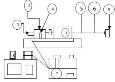
[image:2.595.72.263.354.491.2]

The engine used is a four stroke single cylinder diesel engine. The specifications of the engine are given in Table 1. The schematic diagram of the experimental setup is shown in Fig. 1.

Fig – 1: Schematic diagram of experimental setup

1. Engine 2.Dynamometer 3.Crank angle encoder 4.Load cell 5.Exhaust gas analyzer 6.Smoke meter 7.Control panel 8.Computer 9.Silencer

A pressure transducer is used to monitor the injection pressure. The engine apparatus was connected with an emission measurement device AVL Digas 444 a five gas analyser. The setup is provided with necessary instruments for measuring combustion pressure and crank angle. The signals from the above instruments are interfaced to the computer through engine indicator for P-V and P-Ɵ diagrams with AVL INDIMICRA 602 –T10602A (V2.5). Atmospheric air enters the intake manifold of the engine through an air filter and an air box. An air flow sensor fitted with the air box gave the input for the air consumption to the data acquisition system. All the inputs such as air and fuel consumption, engine brake power, cylinder pressure and crank angle were recorded by the high speed data acquisition system, processed in the computer. A thermocouple in conjunction with a temperature indicator was connected at the exhaust

pipe to measure the temperature of the exhaust gas. The smoke density of the exhaust was measured by the help of an AVL415 diesel smoke meter. A crank position sensor was connected to the output shaft to record the crank angle.

3. Experimental Procedure

To evaluate the performance and emission characteristics, initially the engine was run on zero load condition at standard injection timing of 230 bTDC and injection pressure of 20 N/mm2 at a constant speed of 1500 rpm. In order to change the injection timing, the flywheel is rotated to bring the piston to TDC position. Then the flywheel is rotated in anti-clock wise direction until the fuel reaches the fuel injector. The movement of the flywheel should be noted carefully. The flywheel is rotated back by 5mm and this position is marked on the flywheel for the desired injection timing. Shims are added or removed to adopt the other injection timing positions [20]. In the present study, injection timing is altered to 160, 190, 230 and 250 bTDC position. The fuel injection pressure is changed by adjusting the screw provided above the fuel injector. By tightening the screw, the injection pressure is increased and vice-versa. The desired injection pressure is tested by a fuel injector pressure tester. Eddy current dynamometer is used to impart load on the engine. The current and thus the load is varied by a dimmer stat. The experiments were conducted at 4A, 9A, 13 A and 18A load apart from 0A load.

4. Optimization Using Grey Relational Analysis

In the present study load, fuel injection timing, fuel injection pressure are considered as the major influencing factors. Based on the findings available on open literature, the levels and their ranges were selected.

4.1Selection of level of factors

For the factor fuel injection timing, 160, 190, 230 and 250 before top dead centre (bTDC) are taken as levels. Smoke emission and NOx emission increases with further increase in advancing and retarding the timing [16]. For factor fuel injection pressures, 18, 20, 22 and 24 N/mm2 are chosen as the levels. It is noticed that engine operation was smooth till 24 N/mm2 pressures [17]. For factor load, 4A, 9A, 13A and 18A are taken as levels. The design factors and their levels chosen are shown in the Table 2.

Table 2. Design factors and their levels

Factor No Factor Influencing Level of factor

1 2 3 4

1 Load (A) 4 9 13 19

2 Injection Timing (0_bTDC) ₁₆ ₁₉ ₂₂ ₂₅

(3)

BTE, NOx, HC, CO, CO2 and O2 are analyzed in this study.

4.2 Grey Relational Analysis

Signal-to-noise ratio(S/N) is used in engineering for comparing the level of a desired signal to the level of background noise [18]. The experimental results were normalized in the range between zero and one. For brake power, brake thermal efficiency and O2, the “higher-the-better” original sequence was normalized as follows:

) ( min ) ( max ) ( min ) ( ) ( k y k y k y k y k x i i i i i _   (1) For brake specific fuel consumption, NOx, HC, CO and CO2, the “lower-the-better”. The original sequence was

normalised as follows:

) ( min ) ( max ) ( ) ( max ) ( k y k y k y k y k x i i i i i _   (2)

)

(

k

y

i _{is the original reference sequence,}

x

i

(

k

)

_{is the}

sequence for comparison. i = 1,2,3…..m, k = 1,2,3….n with m,n being total number of experiments and responses.

min

y

i

(

k

)

_{is the smallest value of}

y

i

(

k

)

_{and max}

y

i

(

k

)

_is

the highest value of

y

i

(

k

)

. The grey relational coefficients

were obtained from the normalized experimental data to express the relationship between the desired and actual

experimental data. The grey relational coefficient



i

(

k

)

_is

calculated as, max max min ) ( ) (        k k oi i   (3) where Δoi = ‖ x0(k) - xi(k) ‖ (4)

Δmin , Δmax are the min and max values of absolute differences (Δoi) of all distinguishing coefficient (0 ≤ Ψ ≤ 1). In the present study, the value of Ψ is taken as 0.5 [18].

4.3 Grey relational Generation

The grey relational grade is calculated as,





n k i i o

n

1

1 





[image:3.595.76.526.500.784.2]

And ∑β=1 (5) Where β is the weighting factor.In the present study, the values of weighting factors are taken equally such that the sum of weighting factors is 1. Table 3 shows the Grey relational grade for each experiment.

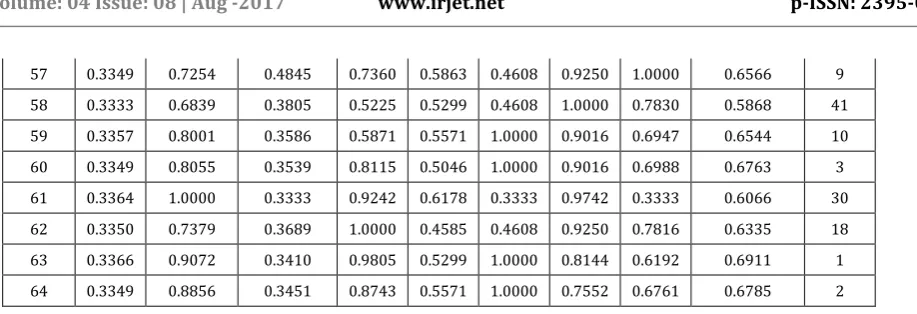
Table 3. Grey relational coefficient & grey relational grade with rank

Exp No.

Grey Relational Coefficient

Grey Relational

Grade Rank BP (kW) BSFC (kg/h kW) BTE

(%) (ppm) NOx (ppm) HC (%) CO (%) CO2 (%) O2

1 1.0000 0.3518 0.6491 0.3478 0.5863 1.0000 0.5422 0.5006 0.6222 23 2 0.9810 0.3385 0.6909 0.3333 0.5299 1.0000 0.5140 0.5006 0.6110 28 3 0.9169 0.3581 0.6142 0.4025 0.4376 0.4608 0.5280 0.5015 0.5255 54

4 0.9257 0.3693 0.6142 0.4945 0.8746 0.4608 0.5280 0.4993 0.5960 38 5 0.9869 0.3333 0.6909 0.4126 0.5299 1.0000 0.5566 0.5402 0.6313 19 6 0.9223 0.3525 0.6491 0.4016 0.4808 1.0000 0.5280 0.4997 0.6043 32 7 0.9869 0.3581 0.6142 0.4822 0.5046 1.0000 0.5422 0.5095 0.6247 20

8 0.9257 0.3693 0.6142 0.5431 0.8746 0.4608 0.5280 0.4993 0.6021 33 9 0.9869 0.3585 1.0000 0.4901 0.4376 1.0000 0.4867 0.5365 0.6620 7 10 0.9169 0.3581 0.6142 0.4369 0.4376 0.4608 0.5280 0.5015 0.5318 53 11 0.9805 0.3595 0.6142 0.4574 0.5046 1.0000 0.5422 0.5095 0.6210 25

(4)

14 0.9632 0.3497 0.6491 0.5699 0.4376 0.4608 0.5280 0.5015 0.5575 46 15 0.9869 0.3581 0.6142 0.5628 0.5046 1.0000 0.5422 0.5095 0.6348 17

16 0.9257 0.3693 0.6142 0.5431 0.8746 0.4608 0.5280 0.4993 0.6021 35 17 0.4854 0.5886 0.4086 0.3819 0.4178 0.4608 0.6494 0.5391 0.4915 63 18 0.4788 0.5146 0.4462 0.3743 0.3646 0.4608 0.6172 0.5391 0.4745 64 19 0.4749 0.5573 0.4169 0.4574 0.4808 0.4608 0.6494 0.5540 0.5064 59

20 0.4778 0.5516 0.4259 0.5369 1.0000 1.0000 0.4471 0.4738 0.6141 26 21 0.4839 0.4746 0.4705 0.4769 0.6887 0.4608 0.6494 0.5886 0.5367 50 22 0.4749 0.5322 0.4356 0.4601 0.6178 0.4608 0.6172 0.5489 0.5184 58 23 0.4832 0.5425 0.4259 0.5835 0.5863 1.0000 0.6331 0.5523 0.6009 37 24 0.4778 0.5516 0.4259 0.5781 1.0000 1.0000 0.3333 0.4738 0.6051 31

25 0.4803 0.5592 0.5591 0.5826 0.5046 0.4608 0.6016 0.5886 0.5421 49 26 0.4749 0.5573 0.4169 0.4557 0.4808 0.4608 0.6494 0.5540 0.5062 60 25 0.4819 0.5443 0.4259 0.5225 0.5863 1.0000 0.6331 0.5523 0.5933 39

28 0.4778 0.5516 0.4259 0.7129 1.0000 1.0000 0.4471 0.4738 0.6361 16 29 0.4809 0.5841 0.4086 0.6863 0.5299 0.4608 0.6830 0.5974 0.5539 47 30 0.4774 0.5516 0.4259 0.6709 0.4808 0.4608 0.6494 0.5540 0.5339 52 31 0.4832 0.5425 0.4259 0.6767 0.5863 1.0000 0.6331 0.5523 0.6125 25

32 0.4778 0.5516 0.4259 0.7129 1.0000 1.0000 0.3459 0.4738 0.6235 21 33 0.3866 0.6909 0.3746 0.4574 0.4376 0.4608 0.6830 0.5540 0.5056 61 34 0.3822 0.6025 0.4008 0.4253 0.3991 0.4608 0.7182 0.5953 0.4980 62 35 0.3783 0.6804 0.3805 0.5130 0.4178 0.4608 0.7552 0.6139 0.5250 55

36 0.3812 0.7422 0.3689 0.5871 0.6887 1.0000 0.7365 0.5981 0.6378 15 37 0.3862 0.6704 0.3805 0.5458 0.6178 0.3333 0.7941 0.6269 0.5444 48 38 0.3773 0.6607 0.3869 0.5289 0.5571 0.3333 0.7365 0.5953 0.5220 57 39 0.3851 0.6770 0.3805 0.6680 0.5046 1.0000 0.7552 0.6037 0.6218 24

40 0.3812 0.7422 0.3689 0.6219 0.6887 1.0000 0.7365 0.5981 0.6422 13 41 0.3832 0.6874 0.4169 0.6359 0.4376 1.0000 0.7365 0.6887 0.6233 22 42 0.3783 0.6804 0.3805 0.4945 0.4178 0.4608 0.7552 0.6139 0.5225 56 43 0.3834 0.6839 0.3805 0.5529 0.5046 1.0000 0.7552 0.6037 0.6080 29

44 0.3812 0.7422 0.3689 0.7953 0.6887 1.0000 0.7365 0.5981 0.6639 5 45 0.3850 0.7466 0.3636 0.8549 0.4178 0.4608 0.8353 0.6677 0.5915 40 46 0.3814 0.6671 0.3805 0.8170 0.4178 0.4608 0.7552 0.6139 0.5617 43 47 0.3851 0.6770 0.3805 0.8335 0.5046 1.0000 0.7552 0.6037 0.6425 12

48 0.3812 0.7422 0.3689 0.7953 0.6887 1.0000 0.7365 0.5981 0.6639 6 49 0.3357 0.8001 0.3586 0.5174 0.5046 0.4608 1.0000 0.5899 0.5709 42 50 0.3351 0.6770 0.3805 0.4972 0.3333 0.4608 0.9016 0.6968 0.5353 51 51 0.3349 0.9225 0.3410 0.5619 0.5299 1.0000 0.8144 0.6192 0.6405 14

52 0.3349 0.8055 0.3539 0.6026 0.5046 1.0000 0.9016 0.6988 0.6502 11 53 0.3335 0.7466 0.3636 0.6518 0.7289 0.3333 0.9250 0.7325 0.6019 36 54 0.3333 0.7173 0.3689 0.6210 0.5571 0.3333 0.8567 0.6907 0.5598 44 55 0.3366 0.7948 0.3586 0.7208 0.5571 1.0000 0.9016 0.6947 0.6705 4

(5)

57 0.3349 0.7254 0.4845 0.7360 0.5863 0.4608 0.9250 1.0000 0.6566 9 58 0.3333 0.6839 0.3805 0.5225 0.5299 0.4608 1.0000 0.7830 0.5868 41

59 0.3357 0.8001 0.3586 0.5871 0.5571 1.0000 0.9016 0.6947 0.6544 10 60 0.3349 0.8055 0.3539 0.8115 0.5046 1.0000 0.9016 0.6988 0.6763 3 61 0.3364 1.0000 0.3333 0.9242 0.6178 0.3333 0.9742 0.3333 0.6066 30 62 0.3350 0.7379 0.3689 1.0000 0.4585 0.4608 0.9250 0.7816 0.6335 18

63 0.3366 0.9072 0.3410 0.9805 0.5299 1.0000 0.8144 0.6192 0.6911 1 64 0.3349 0.8856 0.3451 0.8743 0.5571 1.0000 0.7552 0.6761 0.6785 2

[image:5.595.78.537.70.227.2]

A higher value of grey relational grade shows that the corresponding S/N ratio is closer to the normalized S/N ratio. As shown in Table 3 the experiment number 63 has the best performance characteristics out of 64 experiments as it has the highest grey relational grade. In this way a multiple response process optimization is converted into a single response problem. The effect of each factor on the Grey relational grade at various levels can be independent [19]. The larger the grey relational grade, the better the multiple performance characteristics. However, the most influencing factor on the set objective needs to be known such that the optimal combination of performance parameters can be determined accurately [20]. For better performance and minimum emissions of the engine, the optimum process parameter combination is found to be A4B4C4. i.e., at 18A load, 250 bTDC Injection timing and 24 N/mm2 Injection pressure as shown in Fig 2. The response table for the S/N ratio is shown in Table 4.

Table 4. Response table for grey relational grade

Symbol

Grey Relational Grade

Process Parameter Level 1 Level 2 Level 3 Level 4

A Load 0.599 0.559 0.588 0.630

B Injection timing 0.563 0.571 0.605 0.609

C Injection pressure 0.581 0.547 0.611 0.637

Fig – 2: Effect of process parameters on grey relational grade

5. Analysis of variance (ANOVA)

ANOVA is used to investigate the performance parameter which significantly influences the performance of the engine. The total sum of squares deviations (SST) is calculated by:

SST = Ʃ (ni--m)2 (6)

Where m is the overall mean of the S/N ratio. The total sum of Squared deviations, SST is divided into two sources:

SS

T



(7)

Where SSj is the sum of squared deviations for each design parameter and is given as

SSj = (8)

Where n is the number of significant parameters and l_the

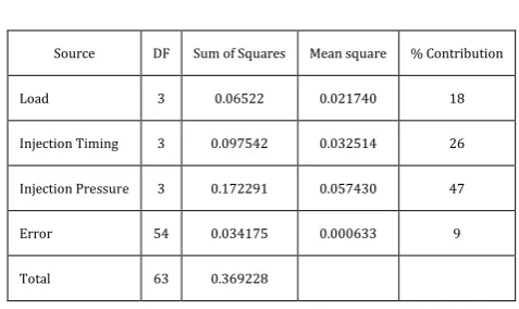
[image:5.595.39.295.478.740.2]

number of levels of each parameter. SSe is the sum of squared error with or without pooled factor, which is the sum of squares corresponding to the insignificant factors. Mean square of a factor (MSj) is found by dividing its sum of squares with its degree of freedom. % contribution (ρ) of each of the design parameter is given by the following equation: ρi = SSj / SST. ANOVA is applied to investigate which factor influences the performance of the engine. The percentage contribution of various factors is shown in Fig 3. The ANOVA table is shown in Table 5. The most significant factor is the fuel injection pressure which contributes 47%.

(6)

[image:6.595.41.280.109.251.2]

Table 5. ANOVA table

Source DF Sum of Squares Mean square % Contribution

Load 3 0.06522 0.021740 18

Injection Timing 3 0.097542 0.032514 26

Injection Pressure 3 0.172291 0.057430 47

Error 54 0.034175 0.000633 9

Total 63 0.369228

6. Confirmation test

The optimum process parameter combination is found to be A4B4C4. i.e., at 18A load, 250 bTDC Injection timing and 24 N/mm2 Injection pressure. In order to verify the actual improvement of the quality characteristic, the confirmation test is conducted for the above combination and was repeated twice. For the prediction of Grey relation αpredicted of the optimal performance parameter, it can be expressed as:

m

predicted





+ (9)

in which, α0 is the average grey relational grade of the optimal level of the significant factor, αm is the average grey relational grade and N is the number of significant factors. The grey relational grade for predicting the optimal performance parameter is computed as 0.688. The evaluation points obtained for BP, BSFC, BTE, NOx, HC, CO, CO2 and O2 were 4.31kW, 0.1983 kg/h kW, 42%, 661ppm, 33 ppm, 0.02%, 4.4%, 13.8% respectively. The S/N ratios of the above parameters were 12.6895, 14.0535, 32.465, 56.4040, -30.3703, 33.9794, -12.8691, and 22.785 respectively. The computational value of Grey relational grade is 0.6939. Table 6 shows the comparison between the initial and optimal process parameter.

Table 6. Comparison between initial and optimal process parameter

Responses

Optimal parameter

Raw Prediction Experiment

A4B4C3 A4B4C4 A4B4C4

BP (kW) 4.287 4.310

BSFC (kg/h kW) 0.206 0.198

BTE (%) 41 42

NOx (ppm) 669 661

HC (ppm) 34 33

CO (%) 0.02 0.02

CO2 (%) 4.1 4.4

O2 (%) 14.23 13.8

Grey relational grade 0.6785 0.6888 0.6939

Percentage improvement in grey relational grade = 2.26%

7. Conclusion

The following conclusions have been derived by applying grey relational analysis to optimize the performance parameters like Load, Injection timing and Injection pressure on a single cylinder diesel engine:

 The experimental results showed that 18A load, 250bTDC and 22 N/mm2 combination is close to the optimal value based on the rank.

 The best performance out of the engine can be obtained at 18A load, 250bTDC injection timing and 24 N/mm2 injection pressure, which is deduced from the Multi response optimization using Grey relational grade.

 Based on ANOVA, fuel injection pressure has a dominant effect of 47% in contribution, while Load has 18% and injection timing has 26% contribution.

An improvement in Grey relational grade of 2.26% can be achieved by the combination.

REFERENCES

[1] Kalaimoorthy, S., Paramasivam,R., 2013. Investigation of

performance and emissions of a biodiesel engine through optimization techniques. Thermal Science. 17, 179-193.

[2] Ganapathy, T., Murugesan, K., Gakkhar, R.P., 2009.

Performance optimization of jatropha biodiesel engine model using Taguchi approach. Applied energy. 86(11), 2476-2486.

[3] Maheswari, N., 2011. A nonlinear regression based multi

objective optimization of parameters based on experimental data from an IC engine fuelled with biodiesel blend. Biomass and bio energy. 35(5), 2171-2183.

[4] Karnwal, A., 2011. Multi response optimization of diesel

engine performance parameters using thumba bio diesel- diesel blends by applying taguchi method and grey relational analysis. International journal of automotive technology. 12(4), 599-610.

[5] Alanso, J.M., 2007. Combining neural networks and

genetic algorithm to predict and reduce diesel engine emission. IEEE Trans Evol. 11(1), 46-55.

[6] Nataraj, M., 2005. Optimizing diesel engine parameters

for low emissions using taguchi method Variation risk analysis approach part 1. Indian journal of engineering and material sciences. 12(6), 169-181.

[7] Anant Bhaskar Garg., 2012. Artificial neural networks

(7)

engineering research. 3(5), 166-170.

[8] Karthikeyan, R., Nallusamy, N., 2010. Optimization of

engine operating parameters for turpentine mixed diesel fuelled DI engine using taguchi method. Modern applied science. 4(12), 182-192.

[9] David Mac Millan., Law, T., Shayler, P., Pegg, I., 2012. The

Influence of Compression Ratio on Indicated Emissions and Fuel Economy Responses to Input Variables for a DI Diesel Engine Combustion System. SAE Technical Paper. 2012-01-0697. doi:10.4251/2012-01-0697.

[10] Ryouta Minamino., Kawabe, T., Omote, H., Okada, S.,

2013. The Effect of Compression Ratio on Low Soot Emission from a Small Non-Road Diesel Engines. SAE Technical Paper. 2013-24-0060. doi:10.4251/2013-24-0060.

[11] Carlo Beatrice., Avolio, G., Del Giacomo, N., Guido, C.,

2008. Compression Ratio Influence on the Performance of an Advanced Single-Cylinder Diesel Engine Operating in Conventional and Low Temperature Combustion Mode. SAE Technical Paper. 2008-01-1678. doi:10.4251/2008-01-1678.

[12] Cursente, V., Pacaud, P., Gatellier, B., 2008. Reduction of

the Compression Ratio on a HSDI Diesel Engine Combustion Design Evolution for Compliance the Future Emission Standards. SAE International Journal of Fuels and Lubricants. 1(1), 420-439. doi: 10.4251/2008-01- 0839.

[13] Hiroshi Sono., Shibata, M., Tajima, Y., Ikeya, K., 2010. A

Study of High Power Output Diesel Engine with Low Peak Cylinder Pressure. SAE Technical Paper. 2010-01-1107.doi:10.4251/2010-01-1107.

[14] Sylvian, Mendez., Thirovard, B., 2009. Using multiple

injection strategies in diesel combustion: Potential to improve emissions, noise and fuel economy trade off in low compression ratio engines. SAE Int Journal fuels Lubricants. 1(1), 662-674. doi: 10.4251/2008-01-1329.

[15] Asad, U., Han, X., Zheng, M., 2011. An empirical study to

extend engine load in diesel low temperature combustion. SAE Intl journal of engines. 5(3), 709-717. doi: 10.4251/2011 – 01-1814.

[16] Payri, F., Benajes, J., Arregle, J., Riesco, J.M., 2006.

Combustion and exhaust emissions in a heavy duty diesel engine with increased premixed combustion phase by means of injection retarding. Oil gas science technology rev IFP.61(2), 247-258.

[17] Jindal, S., Nandwana, B.P., Narendra Rathore., Vinod

Vashistha., 2010. Experimental investigation of the effect of compression ratio and injection pressure in a direct injection diesel engine running on jatropha methyl ester. Applied Thermal Engineering. 30(5), 442-448.

[18] Goutham Pohit., Dipten Misra., 2013. Optimization of

performance and emission characteristics of diesel engine with biodiesel using grey taguchi method. Journal of engineering. doi: 10.1155/2013/915357.

[19] Ranganathan, S., Senthilvelan, T., 2011. Multi response

optimization of machining parameters in hot turning using grey analysis. Intl Journal of advanced manufacturing technology. 56, 455-462. doi: 10.1007/s00170=011-3198-5.

[20] Saravanan, S., Govindan Nagarajan., Santhanam

Optimization of Operating Parameters on a Diesel Engine using Grey Relational Analysis