Varying Response Ratio Priority: A Preemptive CPU Scheduling Algorithm (VRRP)

(1)

http://dx.doi.org/10.4236/jcc.2015.34005

Varying Response Ratio Priority:

A Preemptive CPU Scheduling

Algorithm (VRRP)

Pawan Singh, Amit Pandey, Andargachew Mekonnen

School of Informatics, IOT, Hawassa University, Awassa, Ethiopia Email: [email protected], [email protected]

Received 14 March 2015; accepted 13 April 2015; published 14 April 2015

This work is licensed under the Creative Commons Attribution International License (CC BY). http://creativecommons.org/licenses/by/4.0/

Abstract

In present era, one of the most important resources of computer machine is CPU. With the in-creasing number of application, there exist a large number of processes in the computer system at the same time. Many processes in system simultaneously raise a challenging circumstance of man- aging the CPU in such a manner that the CPU utilization and processes execution gets optimal per-formance. The world is still waiting for most efficient algorithm which remains a challenging issue. In this manuscript, we have proposed a new algorithm Progressively Varying Response Ratio Pri-ority a preemptive CPU scheduling algorithm based on the PriPri-ority Algorithm and Shortest Re-maining Time First. In this scheduling algorithm, the priority is been calculated and the processes with high priority get CPU first or next. For new process, the priority of it becomes equal to inverse of burst time and for the old processes the priority calculation takes place as a ratio of waiting time and remaining burst time. The objective is to get all the processes executed with minimum average waiting time and no starvation. Experiment and comparison show that the VRRP outper-forms other CPU scheduling algorithms. It gives better evaluation results in the form of scheduling criteria. We have used the deterministic model to compare the different algorithms.

Keywords

Operating System, CPU Scheduling, Priority Scheduling, Turnaround Time, Waiting Time, Response Time, Context Switching

1. Introduction

(2)

resources. After a vast advancement of technology, the cost of hardware get reduced to affordable price and the interest of author turned to fast calculation and response. The system is controlled by the multiprogramming and multitasking approach of operating system. The CPU plays an important role in implementation of multipro-gramming and multitasking [1]. The use of computer has affected most of the working of our daily life and the use in almost all sort of field has invited a number of applications for every level of users. As many applications worked simultaneously which required many numbers of processes to be created, the processes must be exe-cuted in such a manner to provide the better response to users. The increment of processes in the system in-creased the responsibility of CPU scheduler. The users expect fast response and execution, and users’ expecta-tion results in a requirement of least waiting time in execuexpecta-tion. There exist a number of scheduling algorithms [2] [3] but Round Robin, Shortest Remaining Time First and the Priority scheduling may have the weightage of the most widely used scheduling algorithms. They have their advantages and disadvantages too. The concept of de-signing a scheduling algorithm has a significant age around thirty years; even then we are motivated to found some scope of improvement in the CPU scheduling approach. We believe that there always exists some hope where normal people found dead, because it depends on the view of researchers. A significant work has been done by many researchers over last two decades but we find a new hope and through this paper a new schedul-ing algorithm Varyschedul-ing Response Ratio Priority is introduced. In this paper, we have tried to collect the advan-tage of Shortest Remaining Time First and Priority by merging them and to eliminate the starvation condition by using indirect aging. In this scheduling algorithm for new processes the decision of allocating the CPU depends similarly as in shortest remaining time first and for the old processes waiting in ready queue decision gets af-fected by the ratio of waiting time and remaining burst time. The main objective of this paper is to provide the scheduling without starvation and average waiting time if not equal to but nearer to the average waiting time of shortest remaining time first. In this manuscript, we use the deterministic model to compare the VRRP to other scheduling algorithms. The next section contains the brief description of some of the most common scheduling algorithms. In Section 3, we have explained the working and calculation of our approach. Section 4 explains the comparative results with some most favourite scheduling and finally our conclusion comes in the Section 5.

2. Related Work

(3)

minimum waiting time, maximum CPU utilization and minimum overhead of context switches [7] [8]. Some of the scheduling algorithms deployed in the operating systems are:

2.1. First Come First Serve (FCFS)

This is the simplest scheduling algorithm where the processes residing in the ready queue are getting the CPU in the order of their arrival to the ready queue. The process which enters first in the ready queue will get the CPU first and the process which enters afterwards will get it sequentially in the arrival order [2]. This scheduling al-gorithm is nonpreemptive once the process get allocated the CPU it will not leave the CPU until it get termi-nated. In this algorithm the ready queue is implemented using FIFO list. The newly arrival processes are added to the rear end and the CPU is allocated to a process at front end or head. The drawback in this algorithm is the high average waiting time.

2.2. Shortest Remaining Time First (SRTF)

In this scheduling algorithm the decision of which process will get the CPU first or next is decided on the basis of remaining burst time means the excess time required for execution of process. The process with less or mini-mum remaining time required for execution will get the chance to get the CPU for execution [2][9]. In this al-gorithm the ready queue is maintained and the process control block of all processes ready to get the CPU is kept in the Ready queue. The processes with minimum burst time will be selected and the CPU will be allocated to that process. If a new processes enters in the system then the priority of all the processes in the ready queue is been evaluated and if the new arrived process has the less burst time with respect to the executing process then the CPU will be switched to the new process by saving the system statistics on the executing process control block and the new selected statistics to the system. If the new process has the burst time greater than the execut-ing process or the processes in the ready queue than this process control block will be queued in the ready queue. In case no new process arrives before the completion of the executing process than another process will be se-lected by finding the minimum burst time of a process. N this way the scheduler keeps on continuing the selec-tion of processes for allocating the CPU for execuselec-tion. This algorithm has a problem that if the small burst time processes keeps on coming into the ready queue the process with big burst time may be suffer with starvation. The SRTF is better for the processes with low CPU burst time only. It has a better low average response time and low average waiting time.

2.3. Priority Scheduling (PR)

In this type of CPU scheduling algorithm there is always the categorization of processes on the basis of some system factors as type of processes. The importance of any process is made by a range of values and any process entering the ready queue gets allocated its importance as priority. This priority value [9] decides the decision of allocating the CPU to a process in such a way that the process with high value of priority will get the CPU first or next. There are two version of it one is preemptive and another is nonpreemptive. The preemptive algorithm is of our interest. In the preemptive scheduling the processes belongs to a category and that category priority is been allocated at the entry to a ready queue and do not change during the whole life time of a process. As soon as the processes enter into the ready queue by allocating its process control block into ready queue it comes along with the priority generated by the system. The scheduler uses to select the process with high priority and allocate the CPU and if new process arrives than the priority of the executing gets compared to new process pri-ority [2]. If the priority of new process has high value than the CPU is been switched to new process by sched-uler and the statistics of system gets saved into its process control block and the statistics of new process control block required to be loaded into the system, to get start executing the new process. If the new process priority is lesser than the executing process will continue executing and the new process has to wait into ready queue for its turn. In this scheduling the overhead of switching does not contain minimum value but less than other, for high priority processes the waiting time and response time have smaller values. In this algorithm the low priority process may be in starvation [10] if high priority processes keep on coming in the ready queue.

2.4. Round Robin Scheduling (RR)

(4)

order in the ready queue and the fix time of CPU is provided to all the processes, this fix duration of CPU time is called time quantum [11]. If the process do not finishes its execution in this time quantum the process has to wait to get the next quantum. The time slice/quantum [12] allocation done by the scheduling in the cyclic order hence named round robin. The data structure used is FIFO queue [2] the process is selected from the head of queue and the new process is added to the rear end of the queue. The selection of the duration of time quantum plays the great role in this scheduling algorithm. The implementer is suggested to take care while deciding for the time quantum. It must be significant with respect to dispatch latency. It never moves to starvation condition and have low response time but with the cost of high waiting time and turnaround time for long processes [13].

2.5. Highest Response Ratio Next (HRRN)

It is a nonpreemptive priority scheduling algorithm [8] where the priority is been allocated to process on the ba-sis of the ratio called response ratio. Where the service time is the CPU burst time required to execute the full process. The intention of the researcher made to increase the priority if the process has to wait.

(

Waiting Time Service Ti

)

Respo me

Ser nse Ratio

vice Time +

= (1)

3. Our Approach: Varying Response Ratio Priority (VRRP)

In this algorithm the base is priority for CPU allocation decision. We used a different approach for calculating the priority of any process named as varying response ratio next. It is a preemptive priority scheduling algorithm. To calculate the priority following proposition is been used:

Proposition 1: In ideal case initially the priority must be proportion to inverse of burst time.

Proposition 2: The priority must be increased with increase in waiting time for old waiting or executing processes to avoid the starvation condition.

Proposition 3: For waiting or executing processes the priority must be calculated as inverse of remaining time rather than the burst time.

Proposition 4: In any case if two or more than two processes have the same priority then their waiting time will be compared, if the waiting time is similar a process arrive first in ready queue get the preference but if the waiting time is not equal then a process with lowest remaining burst time will be the preferred one.

Acronym and abbreviation used:

Priority of any process Pi VRRPPi

Waiting Time of any process Pi WTi

Burst Time of any process Pi BTi

Remaining Burst Time for Execution of process Pi RBTEi

As per Proposition 1: VRRPPi α 1/BTi (only for new processes) (2)

As per Proposition 2: VRRPPi α WTi (only for old or executing processes) (3)

As per Proposition 3: VRRPPi α 1/RBTEi (only for old or executing processes) (4)

By combining all the propositions shown in the Equations (2)-(4) the priority of process i may be formulated and calculated as:

(

)

(

i i

_{) (}

₎

i i

1

for newly arrived processes BT

1 WT

for old waiting or executing processes RBTE

VRRPP 

= +     

(5)

time. The idea of motivation is that processes with small burst time must get the preference over processes with long burst time or processes with small remaining burst time must get the preference over processes with long remaining burst time and to avoid the starvation condition old processes priority must increase with the increase of waiting time. In this the indirect aging is been used in the form of a factor waiting time. If in case two process gain the same priority then their waiting time will be compared. If the processes have same waiting time FCFS will be applied among those processes. If waiting time is different a process with lowest remaining burst time gets the CPU next. If some processes have similar waiting and some different waiting time then group them by waiting time and sort the individual group using FCFS. All the top elements of every group with different wait-ing time will be compared for remainwait-ing burst time a process with lowest remainwait-ing burst time will get the CPU next.

If two processes Pi and Pj gets same priority then

i j

VRRPP =VRRPP (6)

(

i

) (

j

)

i j 1 WT 1 WT RBTE RBTE + +

= (7)

(

)

(

ij

)

ij

1 WT RBTE

RBTE 1 WT

+ =

+ (8)

If WT_i 1 and WT_j1 then WT_i+ ≈1 WT_i putting this value in Equation (8).

(

)

(

ij

)

ij

WT RBTE

RBTE

WT = (9)

There are two possibility first both waiting time are similar second both waiting time are different. In first case if both waiting time are similar

i j i j

WT =WT then RBTE =RBTE

then a process arrived first must get preference so that it may not wait long to complete its task. In second case if both waiting time are different and

i j i j

WT <WT then RBTE <RBTE

Then a process i with low remaining burst time will get the preference because a process with low remaining burst time will have high possibility that it may finish its execution before arrival of new process and will not get context switched.

Algorithm

Assumption: There exist a Job Pool JP = {p1, p2, ⋅⋅⋅, pn} where n number of processes are residing to come in main

memory to get the CPU for execution, and a long term scheduler (LTS) who is taking a process from JP to main memory ready queue Queue at their submission time. At the starting of CPU scheduling the system time (ST) will be zero and it keep on incrementing. P is a set of processes in Queue. The abbreviation and acronym used in the manuscript to formulize the factors affecting the scheduling algorithms.

Throughput Turnaround Time Terminating Time Response Time

Finishing Time of execution for ith time Average Waiting Time

Context Switch Count

– – – – – – – TP TT TerT RT FtEi AvWT CSC

Number of processes Waiting Time Submission Time

Starting Time of execution for ith time Average Turnaround Time

(6)

Input: Queue φ,

Output: WTi, AvWT, RTi, AvRT, TTi, AvTT

P is a set of processes in Queue

begin repeat {

on submission of a process pi to Queue by LTS –

{

if (Queue φ)

{allocate CPU to pi;

RTi = 0; WTi = 0; StEu pi = ST;}

else

{Add pi to Queue;

SubT pi = ST;

for (j = 1 to m) // all process in queue

{VRRPPj =

(

)

(

)

(

)

j j j

1

only for newly arrived processes BT

1 WT

only for old waiting or executing processes RBTE

    +   

;}

Select pk max (VRRPPj, m)

If (pk is not executing and any other pe is executing)

{deallocate CPU from pe;

FtEu pe = ST;

Allocate CPU to pk;

StEu pk = ST;

if (RBTEk = BTk)

{RTk = ST SubT pk;

WTk = ST − SubT pk;}

else

{WTk = WTk + FtEu−1 pk – StEu pk;}sfd

}

else {pk will continue execution}

} }

on termination of a process pi

{

FtEu pi = ST;

TTi = FtEu pi− SubT pi;

Delete the process from Queue; if (|Queue| = 1)

{Allocate CPU to remaining process pk;

StEu pk = ST;

if (RBTEk = BTk)

{RTk = ST − SubT pk;

else

{WTk = WTk + FtEu−1 pk− StEu pk;}

} else if (|Queue| > 1)

(7)

{VRRPPj =

(

)

(

)

(

)

j j j

1

only for newly arrived processes BT

1 WT

only for old waiting or executing processes RBTE

    +   

;}

Select pk max (VRRPPj, m)

Allocate CPU to pk;

StEu pk = ST;

if (RBTEk = BTk)

{RTk = ST − SubT pk;

else

{WTk = WTk + FtEu−1 pk− StEu pk;}

} }

} until (no process submitted && Queue  φ)

for (i = 1 to N) // all processes submitted and completed their execution {

N i i 1

1

AvTT TT

N =

=

∑

;

N i i 1

1

AvRT RT

N =

=

∑

;

N i i 1

1

AvWT WT

N =

=

∑

;

} end;

procedure max (VRRPPi, n)

{ list L = {(Pu, VRRPPu), (Pv, VRRPPv), ···, (Pz, VRRPPz),};

sort L; // (such that VRRPPu > VRRPPv > VRRPPw > ··· > VRRPPz)

if ((Lj.VRRP ≠ Lk.VRRP) && (j ≠ k) && (j, k = 1 to n))

{return Po with max(VRRP);}

else if ((Lj.VRRP = Lk.VRRP)&& (j ≠ k)&& (j, k = 1 to m; 2 ≤ m ≤ n))

{if ((Lj.P.WT = Lk.P.WT) && (j ≠ k)&& (j, k = 1 to m))

{return Po with min(SubT);}

else {make groups G = {G1, G2, ···, Gs} of Li (i = 1 to m) with similar Li.P.WT;

sort Gj (j = 1 to s) in increasing order of Gi.P.SubT;

make group Gf = {G1.TOP, G2.TOP, ···, Gs.TOP};

return Po with min(Gf.P.RBT);}

} }

4. Experimental Analysis

(8)

every set of data we have compared our algorithm with SRTF, FCFS, RR and HRRN.

N i i 1

N TP

TT

=

∑

(10)

TT=TerT SubT− (11)

1

RT=StE −SubT (12)

(

)

m

k 1 k

k 1

WT=RT+

∑

= StE + −FtE (13)

N i i 1

1

AvTT TT

N =

=

∑

(14)

N i i 1

1

AvRT RT

N =

=

∑

(15)

N i i 1

1

AvWT WT

N =

=

∑

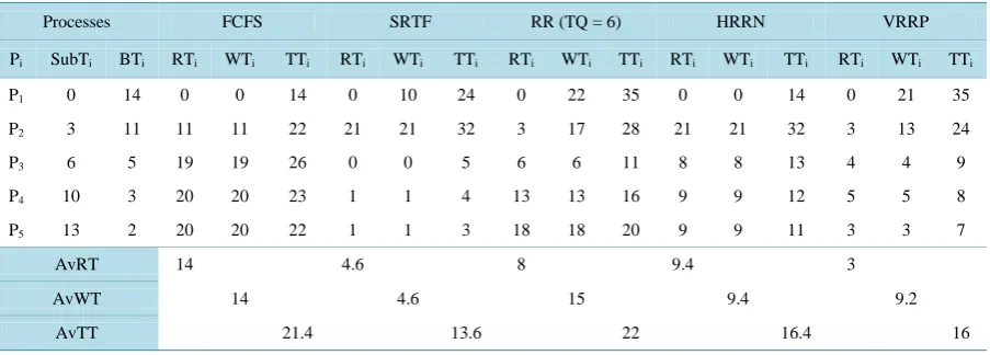
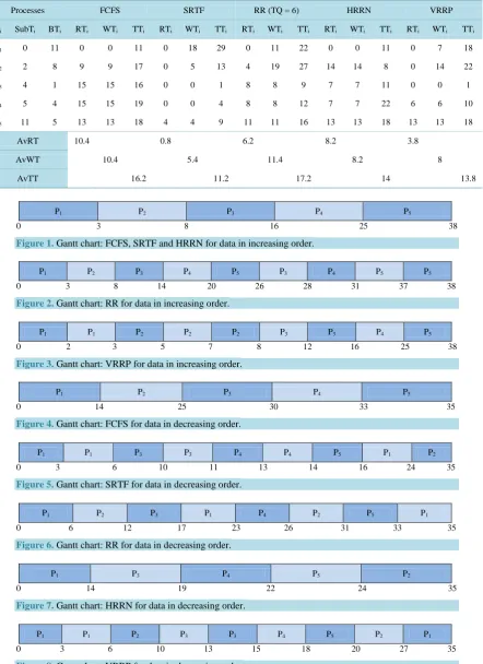
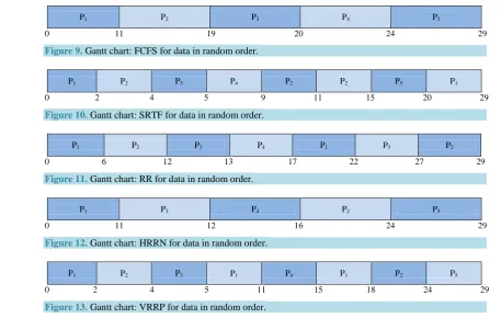
(16)

[image:8.595.88.540.558.720.2]

By using the Equations (1), (5), (10)-(16) the followingTables 1-3 of results are generated and the Gantt chart showing the sequence of process execution for different data and using different algorithms in Figures 1-13.

Table 1. Calculations of factors when the data considered is in increasing order.

Processes FCFS SRTF RR (TQ = 6) HRRN VRRP

Pi SubTi BTi RTi WTi TTi RTi WTi TTi RTi WTi TTi RTi WTi TTi RTi WTi TTi

P1 0 3 0 0 3 0 0 3 0 0 3 0 0 3 0 0 3

P2 2 5 1 1 6 1 1 6 1 1 6 1 1 6 1 1 6

P3 5 8 3 3 11 3 3 11 3 15 23 3 3 11 3 3 11

P4 7 9 9 9 18 9 9 18 7 15 24 9 9 18 9 9 18

P5 12 13 13 13 26 13 13 26 8 13 26 13 13 26 13 13 26

AvRT 5.2 5.2 3.8 5.2 5.2

AvWT 5.2 5.2 8.8 5.2 5.2

AvTT 12.8 12.8 16.4 12.8 12.8

Table 2. Calculations of factors when the data considered is in decreasing order.

P1 0 14 0 0 14 0 10 24 0 22 35 0 0 14 0 21 35

P2 3 11 11 11 22 21 21 32 3 17 28 21 21 32 3 13 24

P3 6 5 19 19 26 0 0 5 6 6 11 8 8 13 4 4 9

P4 10 3 20 20 23 1 1 4 13 13 16 9 9 12 5 5 8

P5 13 2 20 20 22 1 1 3 18 18 20 9 9 11 3 3 7

AvRT 14 4.6 8 9.4 3

AvWT 14 4.6 15 9.4 9.2

(9)

Table 3. Calculation of factors when the data considered is in random order.

P1 0 11 0 0 11 0 18 29 0 11 22 0 0 11 0 7 18

P2 2 8 9 9 17 0 5 13 4 19 27 14 14 8 0 14 22

P3 4 1 15 15 16 0 0 1 8 8 9 7 7 11 0 0 1

P4 5 4 15 15 19 0 0 4 8 8 12 7 7 22 6 6 10

P5 11 5 13 13 18 4 4 9 11 11 16 13 13 18 13 13 18

AvRT 10.4 0.8 6.2 8.2 3.8

AvWT 10.4 5.4 11.4 8.2 8

AvTT 16.2 11.2 17.2 14 13.8

P1 P2 P3 P4 P5

0 3 8 16 25 38

Figure 1.Gantt chart: FCFS, SRTF and HRRN for data in increasing order.

P1 P2 P3 P4 P5 P3 P4 P5 P5

0 3 8 14 20 26 28 31 37 38

Figure 2.Gantt chart: RR for data in increasing order.

P1 P1 P2 P2 P2 P3 P3 P4 P5

0 2 3 5 7 8 12 16 25 38

Figure 3.Gantt chart: VRRP for data in increasing order.

P1 P2 P3 P4 P5

0 14 25 30 33 35

Figure 4. Gantt chart: FCFS for data in decreasing order.

P1 P1 P3 P3 P4 P4 P5 P1 P2

0 3 6 10 11 13 14 16 24 35

Figure 5.Gantt chart: SRTF for data in decreasing order.

P1 P2 P3 P1 P4 P2 P5 P1

0 6 12 17 23 26 31 33 35

Figure 6. Gantt chart: RR for data in decreasing order.

P1 P3 P4 P5 P2

0 14 19 22 24 35

Figure 7. Gantt chart: HRRN for data in decreasing order.

P1 P1 P2 P3 P3 P4 P5 P2 P1

[image:9.595.97.540.101.710.2]

0 3 6 10 13 15 18 20 27 35

(10)

P1 P2 P3 P4 P5

[image:10.595.71.529.80.370.2]

0 11 19 20 24 29

Figure 9. Gantt chart: FCFS for data in random order.

P1 P2 P3 P4 P2 P2 P5 P1

0 2 4 5 9 11 15 20 29

Figure 10. Gantt chart: SRTF for data in random order.

P1 P2 P3 P4 P1 P5 P2

0 6 12 13 17 22 27 29

Figure 11. Gantt chart: RR for data in random order.

P1 P3 P4 P2 P5

0 11 12 16 24 29

Figure 12. Gantt chart: HRRN for data in random order.

P1 P2 P3 P1 P4 P1 P2 P5

0 2 4 5 11 15 18 24 29

Figure 13.Gantt chart: VRRP for data in random order.

As per the graph plotted in the Figure 14when the data sampled is in increasing order our algorithm VRRP provides average response time similar to FCFS, SRTF and HRRN but greater than RR. When the sampled data have decreasing order our algorithm VRRP provides the average response time lesser to FCFS, SRTF, RR and HRRN. When the data selected is random its average response time is less than FCFS, RR and HRRN but great-er than SRTF.

The graph plotted in the Figure 15 reflects that average waiting time of our algorithm VRRP is similar to FCFS, SRTF and HRRN but less than RR if the selected data is in increasing order. When the sampled data is in decreasing order the average waiting time of our algorithm VRRP is lesser to FCFS, RR and HRRN but greater than SRTF. When the data is selected randomly the average waiting time is less than FCFS, RR and HRRN but greater than SRTF.

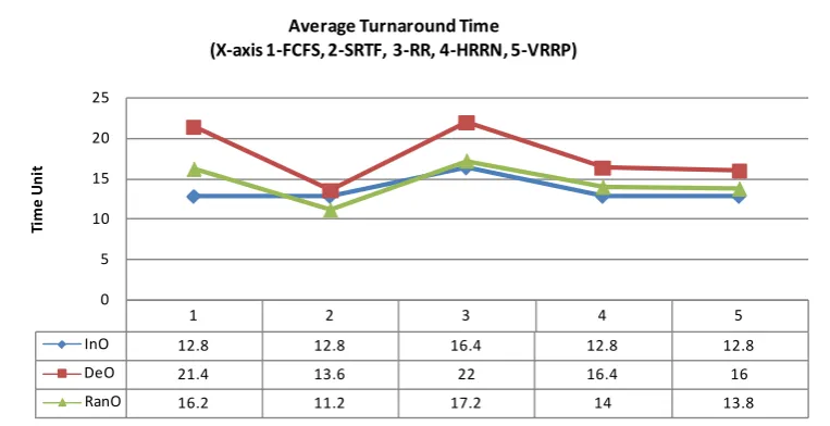
The graph of Figure 16 reflects three cases where the selected data is increasing order, decreasing order and random order. In first case where the data have increasing order our scheduling approach VRRP provides aver-age turnaround time same as FCFS, SRTF and HRRN but less than RR. Secondly when the data have decreasing order or random order our algorithm VRRP calculates average turnaround time less than FCFS, RR and HRRN but greater than SRTF.

The working of VRRP is better than the FCFS and HRRN in all the cases. Although the average response time, average turnaround time and average waiting time of SRTF is better than the VRRP the working of VRRP is better than the SRTF because the SRTF leads to starvation [7] but our VRRP will never let any process in starvation condition. VRRP also provides better results than RR although the average response time of RR is least in case of increasing order of data but its average waiting time and average turnaround time is very high which makes it less efficient.

5. Conclusion

(11)

[image:11.595.124.507.83.269.2] [image:11.595.123.505.295.489.2]

Figure 14. Average response time in increasing, decreasing and random order.

Figure 15. Average waiting time in increasing, decreasing and random order.

Figure 16. Average turnaround time in increasing, decreasing and random order.

1 2 3 4 5

InO 5.2 5.2 3.8 5.2 5.2

DeO 14 4.6 8 9.4 3

RanO 10.4 0.8 6.2 8.2 3.8

0 2 4 6 8 10 12 14 16

Tim

e U

nit

Average Response Time

(X -axis 1-FCFS, 2-SRTF, 3-RR, 4-HRRN, 5-VRRP )

1 2 3 4 5

InO 5.2 5.2 8.8 5.2 5.2

DeO 14 4.6 15 9.4 9.2

RanO 10.4 5.4 11.4 8.2 8

0 2 4 6 8 10 12 14 16

Tim

e U

nit

Average Waiting Time

(X -axis 1-FCFS, 2-SRTF, 3-RR, 4-HRRN, 5-VRRP )

1 2 3 4 5

InO 12.8 12.8 16.4 12.8 12.8

DeO 21.4 13.6 22 16.4 16

RanO 16.2 11.2 17.2 14 13.8

0 5 10 15 20 25

Tim

e U

nit

Average Turnaround Time

[image:11.595.122.504.510.706.2]

(12)

other scheduling algorithms—RR, HRRN and FCFS. In future we can further investigate VRRP—our proposed algorithm—for its usefulness in providing additional task-oriented results in current comprehensive composite functioning of operating system.

References

[1] Stallings, W. (2006) Operating Systems: Internals and Design Principles. 5th Edition, Prentice-Hall, Upper Saddle River.

[2] Silberschatz, A., Peterson, J.L. and Galvin, B. (2006) Operating System Concepts. 7th Edition, Addison Wesley, Bos-ton.

[3] Oyetunji, E.O. and Oluleye, A.E. (2009) Performance Assessment of Some CPU Scheduling Algorithms. Research Journal of Information Technology, 1, 22-26. http://maxwellsci.com/jp/abstract.php?jid=RJIT&no=9&abs=5

[4] Hiranwal, S. and Roy, K.C. (2011) Adaptive Round Robin Scheduling Using Shortest Burst Approach Based on Smart Time Slice. International Journal of Computer Science and Communication, 8, 319-323.

http://www.csjournals.com/IJCSC/IjcscVol2-2.html

[5] Noon, A., Kalakech, A. and Kadry, S. (2011) A New Round Robin Based Scheduling Algorithm for Operating Sys-tems: Dynamic Quantum Using the Mean Average. International Journal of Computer Science Issues, 8, 224-229. http://www.ijcsi.org/contents.php?volume=8&&issue=3

[6] Rajput, S.I. and Gupta, D. (2012) A Priority Based Round Robin CPU Scheduling Algorithm for Real Time Systems. International Journal of Innovations in Engineering and Technology, 1, 1-11.

http://ijiet.com/issues/volume-1-issue-3-october-2012/

[7] Singh, A., Goyal, P. and Batra, S. (2010) An Optimized Round Robin Scheduling Algorithm for CPU Scheduling. In-ternational Journal on Computer Science and Engineering, 31, 2383-2385.

http://www.enggjournals.com/ijcse/issue.html?issue=20100207

[8] Behera, H.S., Swin, B.K., Prinda, A.K. and Sahu, G. (2012) A New Proposed Round Robin with Highest Response Ratio Next (RRHRRN) Scheduling Algorithm for Soft Real Time Systems. International Journal of Engineering and Advanced Technology, 37, 200-206. http://www.ijeat.org/v1i3.php

[9] Tanenbaum, A.S. and Woodfhull, A.S. (2005) Operating Systems Design and Implementation. 2nd Edition, Prentice- Hall, Upper Saddle River.

[10] Shahzad, B. and Afzal, M.T. (2006) Optimized Solution to Shortest Job First by Eliminating the Starvation. Proceed-ings of the 6th Jordanian International Electrical & Electronic Engineering Conference (JIEEEC 2006), Jordan, 14-16 March 2006.

[11] Yadav, R.K., Mishra, A.K., Prakash, N. and Sharma, H. (2010) An Improved Round Robin Scheduling Algorithm for CPU Scheduling. International Journal on Computer Science and Engineering, 24, 1064-1066.

http://www.enggjournals.com/ijcse/issue.html?issue=20100204

[12] Kurzban, S.A., Heines, T.S. and Sayers, A.P. (1986) Operating Systems Principles. 2nd Edition, CBS Publications, New York, 370-371.