http://dx.doi.org/10.4236/am.2015.61007
The Distribution of the Concentration Ratio
for Samples from a Uniform Population
Giovanni Girone, Antonella Nannavecchia Faculty of Economics, University of Bari, Bari, Italy Email: [email protected], [email protected]
Received 24 October 2014; revised 20 November 2014; accepted 16 December 2014 Copyright © 2015 by authors and Scientific Research Publishing Inc.
This work is licensed under the Creative Commons Attribution International License (CC BY). http://creativecommons.org/licenses/by/4.0/
Abstract
In the present paper we derived, with direct method, the exact expressions for the sampling proba-bility density function of the Gini concentration ratio for samples from a uniform population of size n = 6, 7, 8, 9 and 10. Moreover, we found some regularities of such distributions valid for any sample size.
Keywords
Gini Concentration Ratio, Uniform Distribution, Order Statistics, Probability Density Function
1. Introduction
In 1914 Corrado Gini [1] introduced the concentration ratio R for the measure of inequality among values of a frequency distribution. The Gini index is widely used in fields as diverse as sociology, health science, engineer-ing, and in particular, economics to measure the inequality of income distribution.
ased distributions. They showed that these estimators are strongly consistent for the Gini index. Also, they ob-tained an asymptotic normality for the corresponding Gini index.
Girone (1968) [10] focused on the study of the sampling distribution of the Gini index and in 1971 [11] de-rived the exact expression for samples drawn from an exponential population. In 1971 Girone [12] obtained, with direct method, the sampling distribution function of the Gini ratio for samples of size n≤ 5 drawn from a uniform population.
In the present note (Section 2), we calculate the joint probability density function (p.d.f.) of the random sam-ple of size n and, then, the joint p.d.f. of the n order statistics. Hence, we transform one of the order statistics in their average and the remaining n‒ 1 order statistics are divided by the same average. We calculate the joint p.d.f. of the new n variables and integrating with respect to the average we obtain the joint p.d.f. of the other n‒ 1 variables. One of these variables is transformed in the concentration ratio. We calculate the joint p.d.f. of the concentration ratio and of the other n‒ 2 variables and at last we integrate this p.d.f. with respect to the n – 2 va-riables obtaining the marginal p.d.f. of the concentration ratio. The main difficulty of this procedure consists in the identification of the region of integration of the n‒ 2 variables, for two reasons: firstly the need to decom-pose this region into subregions which allow identifying directly the limits of integration and secondly the growing number of such subregions that makes the derivation heavy.
In Sections 3-7, using the software Mathematica, we derive the exact distributions of the concentration ratio for samples from a uniform distribution of size n = 6, 7, 8, 9 and 10. Moreover (Section 8), we find some regu-larities of such distributions valid for any sample size.
2. The Procedure to Derive the Distribution of the Concentration Ratio
Let random variables X X1, 2, , Xn from a uniform population have p.d.f.( )
1, 0 1,0, elsewhere.
x f x = < <
(1) The joint p.d.f. of the variables is
(
1 2)
1, 0 1, for 1,2, , , , , ,
0, elsewhere.
i n
x i n
h x x x = < < =
(2)
The joint p.d.f. of the order statistics X X( )1, ( )2, , X( )n is
( ) ( ) ( )
(
)
( )1 ( )2 ( )1 2
!, 0 1,
, , ,
0, elsewhere.
n n
n x x x h x x x = < < < < <
(3)
By transforming the variables
( )1 ( )2 ( )n,
S X= +X + + X
( )i ( )i , for 1,2, , 1, X
D i n
S
= = −
whose Jacobian is
1,
n
J S= −
we obtain the joint p.d.f. of the variables S and D D( )1, ( )2, , D(n−1) that can be written as
( ) ( ) ( )
(
)
(
)
11 2 1
, , , , 1 ! n ,
n
g s d d d n s −
− = −
(4)
( )1 ( )2 ( 1)
(
( )1 ( )2 ( 1))
for 0<sd <sd <<sdn− <s 1−d −d − − dn− <1.We integrate expression [4] with respect to the variable S and obtain the joint p.d.f. of the variables , , ,
( ) ( ) ( )
(
)
(
)
( ) ( ) ( )
(
)
1 2 1
1 2 1
1 ! , , , , 1 n n n n f d d d
d d d − − − = − − − −
(5)
( )1 ( )2 ( 1) ( )1 ( )2 ( 1) for 0<d <d <<dn− < −1 d −d − − dn− .
By transforming the variable D(n−1) in the variable Ri.e. the concentration ratio
(
)
( ) 1 1 2 1 , 1 n i iR n i D n
−
=
= − −
−
∑
from which we get
( )
(
)(
)
(
)
( ) 2 1 1 1 1 , 2 n n i i n RD − − n i D
=
− −
= −
∑
−the Jacobian of the transformation is
1 2
n
J= −
and the joint p.d.f. of the variable R and D D( )1, ( )2, , D(n−2) is
( ) ( ) ( )
(
)
(
)
(
)(
)
(
)
( )1 2 2 2
1
2 1 !
, , , , ,
2 1 1 2 1
n
n n n
i i
n h d d d R
n R n i d
− − = − = − − − + − −
∑
(6)
for
( ) ( ) ( )
(
)(
)
(
)
( )(
)(
)
(
)
( )2 2
1 2 2
1 1
1 1 1 1
0 1 1 .
2 2
n n
n i i
i i
n R n R
d d d − − n i d − n i d
= =
− − − −
< < << < −
∑
− < − +∑
− − (7)By integrating expression [6] with respect to the variables D D( )1, ( )2 , , D(n−2) over the regions determined
by inequalities [7], we get the marginal p.d.f. of the concentration ratio R.
3. The Distribution of the Concentration Ratio for n = 6
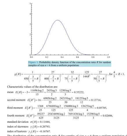
The procedure indicated in Section 2 is used to obtain the following p.d.f. (Figure 1) of the concentration ratio R for random samples of size n = 6:
( )
(
)
2 2 2 2
2 3375 , for
2 1
27 1728 19683 55296 0 1,
5
1 2 3 4
50 25 25 25
5 5 5 5
R
R R R
g
R R
R
− + − + < <
+ + + + + =
( )
1252 7853 2 449523 2 677147 2 55296 2, 1 2,5 5
144 75 1 400 2 225 3 25 4 for
5 5 5 5
R R R R g R R R
− + − + − < <
+ + + +
=
( )
32 2 111312 33773 2 449523 2 19683 2, 2 3,5 5
240
1 1 2 3
75 75
for
400 25
5 5 5 5
R R
R R R R
g R − + − + < <
− + + + +
=
( )
27 2 437 2 111312 7853 2 1728 2, 3 4,5 5
240
2 1 1 2
400 75 75 25
5 5 5 5
for R R R R g R R R
− + − + − < <
− + − + + +
=
Figure 1.Probability density function of the concentration ratio R for random samples of size n = 6 from a uniform population.
( )
1 2 27 2 32 2 1252 27 2,fo 4 1.5 144
3 2 1 1
450 400 75 50
5 5 5 5
r
g R
R R
R
R R R
− + − + < <
− + − + − + +
=
Characteristic values of the distribution are:
mean
( )
3 11696log 2 243log3 1250log5 0.35222,15 2 3
E R = − + + − =
second moment
( )
2 16 69056log 2 24219log3 18125log5 0.13716,25 50 12
E R = − − + =
third moment
( )
3 1368 678688log 2 156006log3 12625log5 0.05785,25 125 125 4
E R = − + + − =
fourth moment
( )
4 89237 25434496log 2 7691436log3 15290log5 0.02606,625 3125 3125 3
E R = − − + =
standard deviation σ
( )
R =0.11444,index of skewness γ1
( )
R =0.20793, index of kurtosis γ2( )
R = −0.16767.The distribution of the concentration ratio R for samples of size n = 6 from a uniform population shows a slight positive skewness and platykurtosis.
4. The Distribution of the Concentration Ratio for n = 7
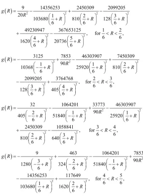
The procedure indicated in Section 2 is used to obtain the following p.d.f. (Figure 2) of the concentration ratio R
for random samples of size n = 7:
( )
(
)
2 2 2 2
2 2
117649 117649 1058841 3764768
1 2 3 4
518400 1620 640 405
6 6 6 6
367653125 1058841 , f 0 1, 6 100 1
5 20736
6
or
R R R R
R R
R
R
g − + − +
+ + + +
− + < <
+ +
Figure 2. Probability density function of the concentration ratio R for random samples of size n = 7 from a uniform population.
( )
2 2 2 22 2
9 14356253 2450309 2099205
20 103680 1 810 2 128 3
6 6 6
49230947 367653125 , 1 2,
6 6
4 5
1620 2
fo 6
6
r 073
6
R
R R R
R R
R g
R
− + −
+ + +
+ − < <
+ +
=
( )
2 2 2 22 2
3125 7853 46303907 7450309
90
1 1 2
10368 25920 810
6 6 6
2099205 3764768 , 2 3,
6 6
3 4
128 405
6
f 6
or
g R
R
R R R
R
R R
− + − +
− + + +
− + < <
+ +
=
( )
2 2 2 22 2
32 1064201 33773 46303907
90
2 1 1
405 51840 25920
6 6 6
2450309 1058841 , 3 4,
6 6
2 3
810 64
for 0
6 6
R
R R R
R g R
R R
− + −
− + − + +
+ − < <
+ +
=
( )
2 2 2 22 2
9 463 1064201 7853
90
3 2 1
1280 324 51840
6 6 6
14356253 117649 , 4 5,
6 6
1 2
103680
fo 162
r 0
6 6
R R
R R
R
R g
R R
− + − +
− + − + − +
− + < <
+ +
( )
2 2 2 22 2
1 9 32 3125
4 3 2 1
8100 1280 405 10368
6 6 6 6
9 117649 , 5 1.
6 20 518 00 1 r
6
o 4
f
g R
R R R R
R R
R
− + −
− + − + − + − +
+ − < <
+
=
Characteristic values of the distribution are:
mean
( )
7 35072log 2 21797log3 359375log5 823543log 7 0.34951,2 15 160 288 1440
E R = − + − + + =
second moment
( )
2 763 3806128log 2 451251log3 359375log5 15647317log 7 0.13291,36 405 80 72 6480
E R = + + − − =
third moment
( )
3 18179 2771144log 2 4266351log3 18546875log5 5764801log 7 0.05417,216 135 320 1728 960
E R = − − − + + =
fourth moment
( )
4 165193 40601588log 2 7638867log3 263234375log5 895191241log 7 0.02342,648 1215 320 15552 77760
E R = + + + − =
standard deviation σ
( )
R =0.10367,index of skewness γ1
( )
R =0.18545, index of kurtosis γ2( )
R = −0.14535.The distribution of the concentration ratio R for samples of size n = 7 from a uniform population shows slight positive skewness and platykurtosis, both lower than those obtained for samples of size n = 6.
5. The Distribution of the Concentration Ratio for n = 8
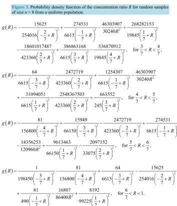
The procedure indicated in Section 2 is used to obtain the following p.d.f. (Figure 3) of the concentration ratio R
for random samples of size n = 8:
( )
(
)
2 2 2 2
2 2 2
8192 2097152 663552 536870912
1 2 3 4
99225 33075 245 19845
7 7 7 7
128000000 169869312 137682944 , 0 1, 7 2025 1
5 6
1323 1225 7
f
7
or
R R R R
R R
R R
g R − + −
+ + + +
+ − + < <
+
+ +
=
( )
2 2 2 22 2 2
16807 9613463 2548367503 386863168 86400 66150 1 423360 2 6615 3
7 7 7
173031518287 19007619787 169869312 , 1 2,
7 7
4 5 6
846720 66150 1225 7
r
7 7
fo
R
R R R
R R
g R
R R
− + − +
+ + +
− + − < <
+ + +
=
( )
2 2 2 22 2 2
81 14356253 31094051 18601017487 120960
1 1 2
490 6615 423360
7 7 7
1969741961 173031518287 128000000 , 2 3,
7 7
3 4 5
13230 846720
for 1323
7 7 7
R
R R R
R
R R
g
R
R − + −
− + + +
+ − + < <
+ + +
=
Figure 3.Probability density function of the concentration ratio R for random samples of size n = 8 from a uniform population.
( )
2 2 2 22 2 2
15625 274531 46303907 268282153
30240
2 1 1
254016 6615 19845
7 7 7
18601017487 386863168 536870912 , 3 4,
7 7
2 3 4
423
for
360 6615 19845
7 7 7
R
R R R
R R
R
R R
g − + − +
− + − + +
− + − < <
+ + +
=
( )
2 2 2 22 2 2
64 2472719 1254307 46303907
30240
3 2 1
6615 423360 6615
7 7 7
31094051 2548367503 663552 , 4 5,
7 7
1 2 3
6615 423360 245
7
r 7
fo 7
g
R
R R R
R R R
R
R
− + −
− + − + − +
+ − + < <
+ + +
=
( )
2 2 2 22 2 2
81 15949 2472719 274531
4 3 2 6615 1
7 7 7 7
14356253 9613463 2097152 , for5 6,
7 7
12
156800 66150 423360
66
0960 1 2
7
150 33 7
7 0 5
R R R R
R R
g R
R
R
− + − +
− + − + − + − +
− + − < <
+ +
=
( )
2 2 2 22 2 2
1 81 64 15625
5 4 3 2
7 7 7 7
81 16807
198450 156800 6615 25
8192 , 6 1.
40
7 86400
1 1
490
7 7
16
for 99225
g
R R R R
R R
R R
R
− + −
− + − + − + − +
+ − + < <
− + +
=
mean
( )
4 3475456log 2 2775303log3 2421875log5 3411821log 7 0.34747,315 560 1008 720
E R = − + + − − =
second moment
( )
2 190 3184576log 2 8776431log3 4140625log5 7882483log 7 0.12985,7 63 392 392 360
E R = − − + + =
third moment
( )
3 6016 658405376log 2 1492752159log3 129921875log5 13596863log 7 0.05160,49 5145 27440 5488 240
E R = − + + − − =
fourth moment
( )
4 145475 3729880384log 2 2307400911log3 533984375log5 9851303log 7 0.02162,343 15435 24010 14406 90
E R = − − + + =
standard deviation σ
( )
R =0.09544,index of skewness γ1
( )
R =0.16867, index of kurtosis γ2( )
R = −0.12824.The distribution of the concentration ratio R for samples of size n=8 from a uniform population shows slight positive skewness and platykurtosis, both lower than those obtained for samples of size n=6 and 7.
6. The Distribution of the Concentration Ratio for n = 9
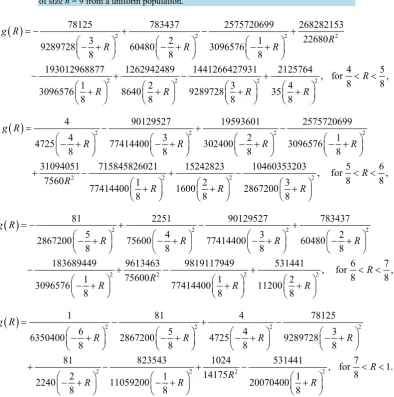
The procedure indicated in Section 2 is used to obtain the following p.d.f. (Figure 4) of the concentration ratio R
for random samples of size n = 9:
( )
2 2 2 22 2 2
2125
531441 531441 10460353203
1 2 3 35 4
8 8 8 8
41518828125 10460353203 437664515463 544195584
5 6 7
764
20070400 11200 2867200
114688 11200 40 00
8 9
8 8 6
R R R R
R R g R R − + − + + + + + − + − + + + + =
(
)
2 for1
, 0 ,
8 1225 1+R < <R
( )
2 2 2 2 22 2
1024 9819117949 15242823 14412664 857395628
77414400 9289728
2867200 9072
27931
14175 1 1600 2 3 945 4
8 8 8 8
6604248318741 2358496602787 437664515463
5 0 6
8 0 8
g R
R
R R R R
R R − + − + + + + + − + − + + = 2 for 409600 1 2 , , 8 8 7 8 R R < < +
( )
2 2 2 22 2 2
823543 9613463 715845826021 1262942489 75600
1 1 2
8 8 8
258217250722
11059200 77414400 8640
309
7 156844988749 6604248318741 104
3 4 5
8 8 8
6576 75600 2867200
R R R g R R R R R − + − + − + + + − + − + + + + = 2
60353203 , 2 3,
8 8 6 11200 8 for R R < < +
( )
2 2 2 22 2 2
81 183689449 31094051 193012968877 7560
1 2 1
2240
8 8 8
2971536239 258217250722
3096576 3096576
857395628 30
7 41518828125
2 3 4 5
8640 945
8 96576 8 8 114688 8
g
R
R R R
R R R R
R − + −
− + − + + + − + − + + + + =
2 fo 3 4
, ,
8 8
r < <R
Figure 4. Probability density function of the concentration ratio R for random samples of size n = 9 from a uniform population.
( )
2 2 2 22 2 2
78125 783437 2575720699 268282153
22680
3 60480 2 1
8 8 8
1
9289728 3096576
2125764 30965
93012968877 1262942489 1441266427931
1 8640 2 3 35 4
8 8 8
76 9 72
8 289 8
R
R R R
R R R
g R − + − +
− + − + − +
− + − +
+ + +
=
2 for 4
5
, ,
8 R 8
R
< <
+
( )
2 2 2 22 2 2
77414400 302400 3096576
4 90129527 19593601 2575720699
4 3 2 1
4725
8 8 8 8
31094051 715845826021 15242823 10460353203 756
77414
0 400 1 1600 2 28672 0 3
8 0
8 8
R R R R
R
R R
g
R
R − + −
− + − + − + − +
+ − + −
+ + +
=
2 fo 5
6
, ,
8 8
r < <R
( )
2 2 2 22 2 2 2
2867200 75600 77414400 6048
81 2251 90129527 783437
5 4 3 2
8 8 8 8
18
0
f 3689449 9613463 9819117949 531441 ,
75600
1 1 11200 2 o
3096576 774144
8 0
8 0 8
R R R R
R
R R R
g R − + − +
− + − + − + − +
− + − +
− + + +
=
6 7 ,
8 r
8
R
< <
( )
2 2 2 22 2 2 2
1 81 4 78125
6 5 4725 4 3
8 8 8 8
81 823543 1024 531441 , 7 1.
8 14175
2 1 1
2
6350400 2867200 9289728
for
11059200 20070400
240
8 8 8
R R R R
R R
R R
g
R
R − + −
− + − + − + − +
+ − + − < <
− + − + +
=
Characteristic values of the distribution are:
mean
( )
9 18425272log 2 1948617log3 1953125log5 109531219log 7 0.34589,2 315 1120 576 5760
E R = − − − + + =
second moment
( )
2 1083 31176874log 2 209048769log3 150390625log5 1101076991log 7 0.12754,32 105 35840 9216 11520
E R = + + − − =
third moment
( )
3 43983 69161579log 2 394860663log3 947265625log5 31654522291log 7 0.04969,256 84 57344 24576 122880
E R = − − + + + =
fourth moment
( )
4 2732815 58613649log 2 36660941253log3 36018359375log5 739122430613log 7 0.02032,4096 35 458752 589824 1474560
E R = + − − − =
standard deviation σ
( )
R =0.08889,index of skewness γ1
( )
R =0.15559, index of kurtosis γ2( )
R = −0.11467.The distribution of the concentration ratio R for samples of size n = 9 from a uniform population shows slight positive skewness and platykurtosis, both lower than those obtained for samples of size n = 6, 7 and 8.
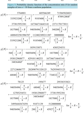
7. The Distribution of the Concentration Ratio for n = 10
The procedure indicated in Section 2 is used to obtain the following p.d.f. (Figure 5) of the concentration ratio R
for random samples of size n = 10:
( )
2 2 2 2 22 2
78125 10000000 234375 5120000000
10287648 321489 4592
762939453125
1 2 56 3 4 5
9 9 9 9 9
450375078125 26214400000
7 734832
30000000
52488 321
00
6 7
7
9 9 489
R R R R R
R g R
R
− + − +
+ + + + +
− + −
+ +
=
(
)
2 46132031252, 0 19,
1568 1 fo
8 9
r R
R R
+ < <
+
+
( )
2 2 2 2 22
59049 6102360983 29486161727807 282890791328125
2508800 1 2 280 3 4
9 9 9 9
112482309211387 781606837730
91871139
64297800 2351462400 94058496
61
5 793800 6
9 85 00
9 91 4
R
R R
g
R R
R
R
− + − + −
+ + + +
+ −
+
=
+ 2 2 2
1465749080718869 2621440000000, 1 2,
9 9
7 for
64297 8
9 9
800 321489
R
R R R
+ − < <
+ +
( )
2 2 22 2 2
32768 9819117949 133551832049 87091200
1 400 1
9 9
34956443674391 227124686777 4488452581986787
2 3 4
1161216
9 9 9
2394237
1148175 9185
68040 335923200
91854
80652283 0
g
R
R R
R R
R
R
− +
− + +
− + −
+ + +
+ =
2 2 2
450375078125, 2 3,
9 9
5 358400 6 7
8684520419229 fo
9
r
0 52488
9 9
R
R R R
− + < <
+ + +
Figure 5.Probability density function of the concentration ratio R for random samples of size n = 10 from a uniform population.
( )
2 2 22 2 2
335923200 9185400
1837
5764801 605566249 715845826021 87091200
2 1
9 9
373815952381 167366716643141 2371170173011
1 2 3
9 9 9
4488452581986787
080 94058496 340200
33
R
R R
R R
g
R
R − + −
− + − +
+ − +
+ + +
− =
2 2 2
112482309211387 , 3 4,
9 9
4 5 7 6
9 9
30000000 for
5923200 9185400
9
R
R R R
+ − < <
+ + +
( )
2 2 22 2 2
2
3 1859135071 4305254531
3 2 1
560
9 9 9
193012968877 429101140253 167366716643141 3483648
94058496 1837080
918540 1 9405 2
9 9
2
8496
680
27124686777 40
28 3
9
R R R
R
R R
g R
R
− +
− + − + − +
− + −
+ +
+ −
+
=
2 2
2890791328125 76293 for
94058496 734
9453125 4
8
5
, ,
9 9
9 32
4 5
9
R
R R
+ < <
+ +
( )
2 2 22 2 2
94058496 68040 94058496
1837
78125 195677 29538353821
4 3 2
9 9 9
12705254531 193012968877 373815952381 3483648
1
080 1837080
940584
1
9 9
349564 96
43674391 2 9
R R R
R
R R
g R
R
− + −
− + − + − +
+ − +
− + +
−
+ =
2 2 2
512000
91871139 for
4
0000 , 5 6,
9 9
3 4
280
9 5927 9
R
R R
+ − < <
+ +
( )
2 2 22 2 2
2
64 404606309 779623
5 4 3
1148175 2351462400 48600
9 9 9
29538353821 4305254531 715845826021 87091200
2 1
94058496 1837080
9 9
133551832049 294 1
9185400 9
R R R
R
R R
R
g R − +
− + − + − +
− + −
− + − +
+ −
+
=
2 2
86161727807 234375 , 6 7,
9 9
2 3
2351462400 56
9 9
for R
R R
+ < <
+ +
( )
2 2 22 2 2
2
3 180731 404606309
6 5 4
2508800 64297800 2351462400
9 9 9
195677 1859135071 605566249
3 2 1
68040 94058496 9185400
9 9 9
9819117949 6102360983 87091200
6
R R
g R
R
R R R
R
− + −
− + − + − +
+ − +
− + − + − +
− +
=
2 10000000 2, 79 89,
1 2
4297800 32148
fo 9
9 9
r R
R R
− < <
+ +
( )
2 2 22 2 2
2 2
1 3 64
7 6 5
257191200 2508800 1148175
9 9 9
78125 3 5764801
4 3 2
94058496 560 335923200
9 9 9
32768 59049 78125
2508800
1 1
1148175 10287648
9 9
R R R
R R R
R R
g R
R
− +
− + − + − +
− + −
− + − + − +
+ − +
=
− + +
2
8
, for 1.
9< <R
Characteristic values of the distribution are:
mean
( )
5 686419424log 2 88683579log3 60546875log5 40353607log 7 0.34462,2835 1120 6048 810
E R = − + − + − =
second moment
( )
2 4977475650505 5506009449897293log 2 3870789417061723log31666598976 57868020 115736040
23520914453125log5 155338805614063log 7 0.12574,
5143824 8266860
E R = − + −
+ − =
third moment
( )
3 56500 302665066912log 2 1609375311log3243 76545 1120
99482421875log5 133852914419log 7 0.04823,
489888 174960
E R = − + −
+ − =
( )
4 6581554 10398297681152log 2 1892901777log3 10382748828125log56561 1240029 560 19840464
1189583980753log 7 0.01933, 787320
E R = − + −
+ =
standard deviation σ
( )
R =0.08352,index of skewness γ1
( )
R =0.14505, index of kurtosis γ2( )
R = −0.10366.The distribution of the concentration ratio R for samples of size n = 10 from a uniform population shows slight positive skewness and platykurtosis, both lower than those obtained for samples of size n=6,7,8 and 9.
8. Some Regularities of the Distributions
The analysis of the p.d.f. for n=2,3, ,10 shows some regularities:
● The p.d.f. of the concentration ratio R, for 0< <R 1n and for samples of size n, can be expressed by
( )
( )
(
)
(
)
1 1
1
2 2
1
2
1 1
1 ; 1 !
1
n i
n
i
n n n
i g R
n i
n R
n
− +
− =
−
− −
−
=
−
− +
−
∑
● Furthermore, the p.d.f. of the concentration ratio R, for
(
n−1)
n R< <1 and for samples of size n, can be expressed by( )
( )
(
)
(
)
1 1
1
2 2
1
2
1 1
1 ; 2
1 ! 1
n i n
n
i
n
n i
i g R
i
n R
n
+ − −
− =
−
− + −
−
=
−
− +
−
∑
● The density of the concentration ratio R, for 0< <R 1n and for samples of size n, is given by
( )
(
)
2 1
2
0 d 1 ! ;
n
ng R R n
n
−
= −
∫
● The density of the concentration ratio R, for
(
n−1)
n R< <1 and for samples of size n, is given by( )
(
)
1
1 d 1 2;
1 !
n n
g R R n
− =
−
∫
● The jth term of the density of the concentration ratio R, denoted as ai j, , verifies the following symmetry
, ,.
i j j i
a =a
The coefficients of the ai i, terms of the p.d.f. of the concentration ratio R for samples of size n−1 multip-lied by
(
n−1)
n become the coefficients of the ai+ +1, 1i terms of the same p.d.f. for sample of size n.These results are valid for every sample size and may allow reducing the heavy calculation to determine the p.d.f. of the concentration ratio R.
9. Concluding Remarks
In the present paper we obtain the distributions of the Gini concentration ratio R for samples of size 6,7,8,9 and 10
mean and expressed in terms of the concentration ratio R for the values assumed in each of such regions. The calculation of the limits of integration is particularly heavy and requires a very long processing time.
The obtained results show that the p.d.f. of the concentration ratio R is given by hyperbolic splines with de-gree 2 and with nodes in k n
(
−1)
for k=1,2, ,n−1. Such distributions are unimodal with mean tending to 1 3, which is the value of the concentration ratio R for the population, and have decreasing standard deviation. Moreover, the distributions show a slight positive skewness and platykurtosis that tend to decrease as n increas-es.Beyond the possibility to obtain similar results for samples of larger size, open problems are the derivation of the exact expression for the mean and the other features of the distribution of the concentration ratio R for ran-dom samples of size n drawn from a uniform population.
References
[1] Gini, C. (1914) L’ammontare e la composizionedellaricchezzadellenazioni. Bocca, Torino.
[2] Hoeffding, W. (1948) A Class of Statistics with Asymptotically Normal Distribution. Annals of Mathematical Statistics,
19, 293-325.
[3] Glasser, G.J. (1962) Variance Formulas for the Mean Difference and the Coefficient of Concentration. Journal of the American Statistical Association, 57, 648-654. http://dx.doi.org/10.1080/01621459.1962.10500553
[4] Cucconi, O. (1965) Sulla distribuzionecampionaria del rapporto R di concentrazione. Statistica, 25, 119.
[5] Dall’Aglio, G. (1965) Comportamentoasintoticodellestimedelladifferenza media e del rapporto di concentrazione. Me-tron, 24, 379-414.
[6] Deltas, G. (2003) The Small-Sample Bias of the Gini Coefficient: Results and Implications for Empirical Research.
Review of Economics and Statistics, 85, 226-234. http://dx.doi.org/10.1162/rest.2003.85.1.226
[7] Barrett, G.F. and Donald, S.G. (2009) Statistical Inference with Generalized Gini Indices of Inequality, Poverty, and Welfare. Journal of Business & Economic Statistics, 27, 1-17. http://dx.doi.org/10.1198/jbes.2009.0001
[8] Davidson, R. (2009) Reliable Inference for the Gini Index. Journal of Econometrics, 150, 30-40.
http://dx.doi.org/10.1016/j.jeconom.2008.11.004
[9] Fakoor, V., Ghalibaf, M.B. and Azarnoosh, H.A. (2011) Asymptotic Behaviors of the Lorenz Curve and Gini Index in Sampling from a Length-Biased Distribution. Statistics and Probability Letters, 81,1425-1435.
http://dx.doi.org/10.1016/j.spl.2011.04.013
[10] Girone, G. (1968) Sulcomportamentocampionariosimulato del rapporto di concentrazione. Annalidella Facoltà di Economia e Commerciodell’Universitàdegli Studi di Bari, 23, 5-11.
[11] Girone, G. (1971) La distribuzione del rapporto di concentrazione per campionicasuali di variabiliesponenziali. Studi di Probabilità, Statistica e Ricercaoperativa in onore di Giuseppe Pompilj, Oderisi, Gubbio.