An Efficient Denoising Model based on Wavelet and Bilateral Filters

An Efficient Denoising Model based on Wavelet and

Bilateral Filters

Sudipta Roy

Nidul Sinha

Electrical Engineering Department National Institute of Technology

Silchar - 788010

Asoke K. Sen

Assam University, Silchar - 788011

ABSTRACT

This paper investigates different models developed through hybridization of wavelet and bilateral filters for denoising of variety of noisy images. Hybridization between wavelet thresholding and bilateral filter is done in different configurations. The models are experimented on standard images like Lena, Barbara, Einstein and satellite as well as astronomical telescopic images and their performances are evaluated in terms of peak signal to noise ratio (PSNR) and image quality index (IQI). Out of number of trial models developed, only 25 models are reported as the performance of the rest models are too poor to be reported. Results demonstrate that use of bilateral filters in combination with wavelet thresholding filters in different ways on decomposed subbands deteriorates the performance. But the application of bilateral filter before or after or both before and after decomposition enhances the performance. Specifically, the filter developed with bilateral filter before decomposition of an image is found to give uniform and consistent results on all the images.

General Terms

Keywords

Image denoising, wavelet transform, wavelet thresholding, bilateral filter.

1.

INTRODUCTION

The success of the modern age applications like video broadcasting, the medical imaging or the technological research in telescopic imaging, satellite imaging or geographic information system totally depend on the quality of the digital images [1].

There are different sources of noise that may contaminate any digital image and degrade the quality. The overall noise characteristics in an image depends on many factors, namely type of sensor, pixel dimensions, temperature, exposure time, and ISO speed of the sensor [2]. Among those, dark current noise is generated due to the thermally generated electrons at sensor sites. It is proportional to the exposure time and highly dependent on the sensor temperature. Shot noise has the characteristics of Poisson distribution. It is generated due to the quantum uncertainty in the generation of photoelectron. Amplifier noise and quantization noise occur during the conversion of number of electrons to pixel intensities. Imperfect instruments, problems with the data acquisition process, and interfering natural phenomena also can cause the degradation. Moreover, noise can be generated by transmission errors and compression [1].

Noise is also colour or channel dependent. Typically, green channel is the least noisy whereas blue channel is the noisiest.

In single-chip digital camera, demosaicking algorithms are used to interpolate missing color components. That means in general noise is not white. Noise in a digital image has low-frequency as well as high low-frequency components. Though the high-frequency components can easily be removed, it is very challenging to eliminate low frequency noise as it is difficult to distinguish between real signal and low-frequency noise. Most of the natural images are assumed to have additive random noise, which is modeled as Gaussian type. Speckle noise [3] is observed in ultrasound images, whereas Rician noise [4] affects MRI images. Thus, denoising is often a necessary and the first step to be considered before the image data is analyzed. It is necessary to apply an efficient denoising technique to compensate for any data corruption. The goal of denoising is to remove the noise while preserving the important image features as much as possible.

Linear filtering techniques, such as Wiener filter or match filter, have been used for this purpose for many years. But linear filters may result in some problems, such as blurring sharp edges, destroying lines and other fine image details, and fail to effectively remove heavy tailed noise. This calls for alternatives, like nonlinear filtering. Many literatures [5-7] have emerged on image denoising using nonlinear filters. Thresholding algorithm in an orthogonal transform domain, such as subband or wavelet transform, is a nonlinear filter. Subband transform with orthogonal perfect reconstruction filter-banks is an orthogonal transform. It is known that the subband filters act as a set of discrete time based functions in a vector space and the decomposition of signal is just to project the signal onto these base functions. As for a signal with noise, there are some differences between the coefficients of original signal and noise because of their different features. In general, if an orthogonal transform with high-energy compaction and de-correlation properties is used, most of the energy of the original signal will be compacted into a few high magnitude coefficients [8, 9]. If the image data is corrupted by additive white noise, components that correspond to noise will be distributed among low magnitude high frequency components. Most of the coefficients of noise are of smaller amplitudes. So, it is reasonable to eliminate the noise by comparing all the coefficients with a threshold and cutting off those coefficients with smaller than the threshold values [10, 11].

variations in low frequency and abrupt temporal changes in high frequency [12].

Many denoising methods have been proposed over the years, such as the Wiener filter, wavelet thresholding [11], anisotropic filtering [13], bilateral filtering [14], total variation method [15], and non-local methods [16]. Among these methods, wavelet thresholding has been reported to be a highly successful method. In wavelet thresholding, a signal is decomposed into approximation (low-frequency) and detail (high-frequency) subbands, and the coefficients in the detail subbands are processed via hard or soft thresholding [10, 11, 17, 18]. The hard thresholding eliminates (sets to zero) coefficients that are smaller than a threshold while the soft thresholding shrinks the coefficients that are larger than the threshold also. The main task of the wavelet thresholding is selection of the threshold and the effect of denoising depends on the selected threshold: a bigger threshold will throw off the useful information and the noise components at the same time while a smaller threshold cannot eliminate the noise effectively. Donoho [11] gave a general estimation method of threshold, but the best threshold cannot be found by this method. Chang et al. [19] have used predictive models to estimate the threshold. It is a spatially adaptive threshold based on context modeling. They also presented data-driven threshold for image denoising in a Bayesian framework [20]. In the SURE Shrink approach [18], the optimal threshold value based on the Stein’s Unbiased Estimator for Risk (SURE) is estimated. A major strength of the wavelet thresholding is the ability to treat different frequency components of an image separately; this is important, because noise in real scenarios may be frequency dependent. But, in wavelet thresholding the problem experienced is generally smoothening of edges.

The bilateral filter was proposed in [14] as an alternative to wavelet thresholding. It applies spatial weighted averaging without smoothing edges. This is achieved by combining two Gaussian filters; one filter works in spatial domain, the other filter works in intensity domain. Therefore, not only the spatial distance but also the intensity distance is important for the determination of weights [2]. Hence, these types of filters can remove the noise in an image while retaining the characteristics of the image. However, the filter may not be very efficient in removing noise in the texture part of the image. It also can not remove salt and pepper type of noise. Along with this, there is no theoretical works on the optimal values of the filter parameters.

In this work a hybrid denoising method is proposed to find the best possible solution, so that PSNR and IQI [21, 22] of the image after denoising are optimal. The proposed approach to denoise an image is based on wavelet thresholding and bilateral filtering, which exploits the potential features of both wavelet thresholding and bilateral filter at the same time their limitations are overcome.

In view of the above the main objectives of the work are:

(i) To develop hybrid filters through hybridization of wavelet thresholding and bilateral filters in different configurations and to tune the different parameters of the hybrid filters to optimize the performance of the tuned hybridized filters for denoising different types of images.

(ii) To tune the parameters of the wavelet based filter and bilateral filter individually to optimize their performance for filtering the same types of images as in step (i).

(iii) To compare the performance of the filters developed in step (i) with those in step (ii) in denoising different types of images.

The paper is organized as follows: Section 2 introduces the concept of wavelet thresholding and works on it. Section 3 explains concepts of bilateral filtering along with its workings. Performance measurement criteria are discussed in section 4. Section 5 describes the proposed hybrid denoising model. Experimental results & discussions are given in section 6. Finally the conclusions are drawn in section 7.

2.

WAVELET DECOMPOSITION

A wavelet is simply a small wave, which has its energy concentrated in time to give a tool for the analysis of transient, non-stationary or time varying phenomena.

Generally, in signal processing, the way of representing a signal should be such that the task of extracting certain properties of the signal is important for specific application, like denoising. Also, the building blocks required for processing and representing a signal with a given accuracy, are as few as possible for faster computation. Another important aspect in signal processing especially, image processing, are the detail features, which are dependent on different scales of resolution. Multi-resolution representation as in wavelet decomposition enables one to analyze different details at different resolution scales.

The wavelet decomposition process involves three basic steps as follows:

a linear forward wavelet transform nonlinear thresholding step and a linear inverse wavelet transform

2.1

Wavelet Thresholding

It has been observed that in many signals, energy is mostly concentrated in a small number of dimensions and the coefficients of these dimensions are relatively large compared to other dimensions or to any other signal (specially noise) that has its energy spread over a large number of coefficients. Hence, in wavelet thresholding, each coefficient is thresholded by comparing against a threshold to eliminate noise, while preserving important information of the original signal [23]. Usually two types of thresholding techniques are used:

• Hard thresholding: Hard threshold is a “keep or kill” procedure and is more intuitively appealing.

• Soft thresholding: Soft thresholding shrinks coefficients above the threshold in absolute value.

2.2

Procedure of Wavelet Thresholding

w = Wg = Wf + Wn (1)

Thresholding the wavelet coefficients to obtain the estimate of the wavelet coefficients of ̂: ̂

(2)

Inverse transform the modified coefficients to obtain the denoised estimate ̂ ̂.

(3)

as larger value may result into loss of information while smaller one may allow noise to continue. The proper value of threshold can be determined in many ways. The different methods that are used for the determination of the threshold value are given below:

Universal thresholding Visu Shrink

Sure Shrink Bayes Shrink

The thresholding techniques have some underlying disadvantages. For instance, the estimated wavelet coefficients by the hard-thresholding method are not continuous at the threshold λ which may lead to the oscillation of the reconstructed signal. In the soft-thresholding case, there are deviations between image coefficients and thresholded coefficients which directly influence the accuracy of the reconstructed signal. Retention of the edges is also a problem here. Different edge detection algorithm may be used to extract the contour feature of cell images. Bilateral filter may help to achieve the target of edge retention.

3.

BILATERAL FILTER

The bilateral filter was proposed in [14] as an alternative to wavelet thresholding for image denoising. It applies spatial weighted averaging without smoothing edges. This is achieved by combining two Gaussian filters; one filter works in spatial domain, the other filter works in intensity domain. Therefore, not only the spatial distance but also the intensity distance is important for the determination of weights. At a pixel location x, the output of a bilateral filter can be formulated as follows:

̅( ) ∑ || || ( ) | ( ) ( )| _{( )} (4)

where σd and σr are parameters controlling the fall-off of

weights in spatial and intensity domains, N(x) is a spatial neighborhood of pixel I(x), and C is the normalization constant: ∑ || || ( ) | ( ) ( )| (5)

One weakness of the bilateral filter is not being able to remove salt-and-pepper type of noise. A second drawback of the bilateral filter is its single resolution nature. Unlike the wavelet filter, the bilateral filter may not access to the different frequency components of a signal. Although it is effective in removing high-frequency noise, the bilateral filter fails to remove low-frequency noise. Another issue with the bilateral filter is that there is no theoretical work on the optimal values of the parameters, σd and σr.

3.1

Parameter Selection for the Bilateral

Filter

There are two parameters that control the behavior of the bilateral filter. Referring to eqn. (4), σd and σr characterizes

the spatial and intensity domain behaviors, respectively. Although these parameters should be related to the noise and image characteristics, the issue has not been studied in a length.

In this work, empirical study is carried out to find the optimal parameter values. White Gaussian noise is added to some standard images as well as to some unpublished images and all the images are denoised by applying the bilateral filter with

different values of the parameters σd and σr for evaluating the

performance of the filter.

4.

MEASUREMENT OF

PERFORMANCE

The performance of the denoising technique is judged by using the objective criteria.

For objective measurement, Mean Squared Error (MSE) and Peak Signal to Noise Ratio (PSNR) are used here. Good PSNR does not imply that the visual quality of the image is good. To overcome this problem Image Quality Index (IQI) [22] is considered as the second parameter for judging the quality of denoised images.

MSE may be defined by eqn. (6).

∑ ( )

(6)

where M is the number of elements in the image.

The PSNR may be defined by eqn. (7) as given below:

(( ))

(7)

where n is the number of bits per symbol.

The Image Quality Index (IQI), Q, is proposed by Wang and Bovik [22] as a product of three different factors: loss of correlation, luminance distortion, and contrast distortion and is defined as

̅ ̅ ̅ ̅ (8) where ̅ ∑ ̅ ∑ ∑ ( ̅) , ∑ ( ̅) ∑ ( ̅)( ̅)

The first component of eqn. (8) is the correlation coefficient between f and g, which measures the degree of linear correlation between f and g and its dynamic range is [-1,1]. The second component, with a value range of [0,1], measures how close the mean luminance is between f and g. σf and σg

can be viewed as estimate of the contrast of f and g, so the third component with a value range of [0,1] measures how similar the contrasts of the images are.

Thus, Q can be rewritten as

̅ ̅

( )( ̅ ̅ )

(9)

The dynamic range of Q is [-1,1]. The best value 1 is achieved, if and only if, for all i=1,2,…,M. The lowest value of -1 occurs when ̅ for all i=1,2,…,M.

5.

PROPOSED APPROACH

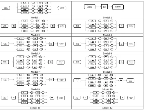
Different hybridized models have been designed and labeled as Model no 4 to 28 in Table 1.

The models investigated in this study fall into four different categories:

i) Model with Wavelet based denoising method only (model no 1).

ii) Model with Bilateral filter only (model no 2).

iii) Model proposed by Ming Zhang and Bahadur Gunturk (Zhang-Gunturk method) (model no 3).

iv) Hybridized models (model nos 4 to 28) in different configurations.

Though initially 48 models were framed and programmed, 25 models are reported here as the performance of unreported models are comparatively very poor.

While designing a model, the parameters w, σd and σr of

bilateral filters are varied over a wide range of values as there is no explicit rules that can guide the tuning of these parameters and the threshold value for the wavelet based filter is also varied.

At the time of construction of the models, the following facts are considered:

i) Different standard available images along with some unpublished images are considered throughout this work. All the models are applied on each and every image.

ii) For a particular image and a model, a wide range of values for w, σd and σr are considered.

iii) After wavelet decomposition, soft thresholding or bilateral technique is applied on each and every subband of the image.

iv) The value of soft thresholding cut off is also considered as a variable here to get the best result with the suitable models.

The PSNR is calculated by eqn. (7) and IQI by eqn. (9) for all the considered models with the considered parameters as discussed above.

Table 1: Different Working Models



Model 1 Model 2

Model 3 Model 4

Model 5 Model 6

Model 7 Model 8

Model 9 Model 10

Model 11 Model 12

Model 13 Model 14

Model 15 Model 16

Model 17 Model 18

Model 19 Model 20

Model 21 Model 22

Model 23 Model 24

Model 25 Model 26

Model 27 Model 28

Table 2: Performance table for the best 6 models

Image Name

Quality

Parameter Model 1 Model 2 Model 3 Model 9 Model 18 Model 19 Lena

PSNR 35.1217 38.3243 30.4803 40.6265 38.6548 39.5561 IQI 0.9222 0.926 0.9465 0.9683 0.9541 0.9664 Barbara

PSNR 34.9942 39.2712 17.5528 40.311 39.7834 39.6969 IQI 0.9464 0.954 0.908 0.9777 0.9677 0.9777 Einstein

PSNR 35.0108 38.3424 24.9062 32.9937 39.4389 39.587 IQI 0.9358 0.9677 0.9386 0.98 0.9696 0.974 Pyramid

PSNR 34.2453 38.7753 12.309 36.9293 39.3131 39.7432 IQI 0.9925 0.9953 0.7857 0.9969 0.9979 0.9976 Astro1 PSNR 35.1464 39.3953 4.9742 34.9593 36.837 39.8931

IQI 0.8666 0.7698 0.3355 0.8227 0.9998 0.8539 Astro2 PSNR 35.121 39.3918 5.7261 35.1238 35.4243 39.67

IQI 0.8903 0.9058 0.5833 0.9276 0.8905 0.9359

6.

EXPERIMENTAL RESULTS AND

DISCUSSIONS

The first model is developed with wavelet based thresholding algorithm [24]. In this algorithm, the images are decomposed into four subbands. The soft thresholding method is then employed on each of the four subbands by varying the thresholding values from 0.001 to 0.1 and the best thresholding result is found with the threshold value as 0.01. Though lowering of thresholding value below 0.01 yields better PSNR but the visual qualities of the denoised images are not as good as with the threshold value of 0.01. The second model is the bilateral filter [4]. The parameters, w, σd

and σrare tuned for finding the optimal performance. The

parameter, σd is varied from 0.01 to 2.2, the window size, w, is

varied from 1 to 11, and σr is varied from 10 to 60. The third

one is the model proposed by Ming Zhang and Bahadur Gunturk [2]. As proposed by the authors, the images are decomposed into four subbands and the both wavelet based and bilateral filters are used as given in model no. 3 in Table 1.

The models from four to twenty eight are the newly designed hybridized ones for the experimentation. For these models, the value of soft-thresholding is set at the same value obtained for model no. 1 with wavelet thresholding only. The parameters, w, σd and σr are varied from 0.01 to 2.2, 1 to 11, and 10 to 60

respectively as considered for the model no. 2.

All the models are experimented with standard pictures like Lena, Barbara, Einstein, satellite picture like Pyramid and two astronomical telescopic images Astro1 and Astro2.

The models 1, 2, 3, 9, 18, and 19 have been found to be well capable in denoising all the images as compared to other models. However, there is some difference in the performance of these six models in terms of PSNR and IQI.

For standard image Lena, model 9 achieved the best PSNR as well as IQI values very closely followed by model 19. Models 18, 2, 1 and 3 follow in descending order in terms of PSNR as is evident in figs. 1 and 2 and in table 3. In the case of Barbara, again the performance of the model 9 is the best in terms of PSNR but in terms of IQI, the performance of model 19 is at par with model 9. For image Einstein, model 19 generates the best PSNR whereas model 9 generates best IQI.

When the satellite image, Pyramid is considered, the best model in terms of PSNR and IQI is 19 followed by model 18.

Models 2 and 9 follows them but the performance of the other two models (1 & 3) are comparatively poorer.

For two astronomical telescopic images, Astro1 and Astro2, model 19 gives the best results, except model 18 that achieves better IQI for image Astro1 even though its PSNR is less.

Model nos. 3 is behaving in a very inconsistent manner. Even though its performance is well for standard images, in case of satellite image the performance deteriorates with further fall in performance for astronomical telescopic images.

Model nos. 27 and 28 are not performing well for all the images.

From the above discussion and the structure of the models, it is observed that in the models whose performance is not good enough are having bilateral filtering technique in the decomposed frequency subbands.

From the results of the experiments in terms of PSNR and IQI as reported in Table 2, the models 9, 18 and 19 of Table 1 are considered as the better models than the other ones.

In model 9, the images are decomposed first into four subbands. In this level the wavelet based soft thresholding is applied on all the subbands. The results obtained after thresholding are then used to reconstruct the image. In the next level, bilateral filter is applied to get the final denoised image.

In model 18, first the image is denoised with bilateral filter followed by decomposition into four subbands. And wavelet thresholding is applied on all the subbands as applied in model 9. The results obtained after thresholding are then used to reconstruct the image. In the last level, again bilateral filter is applied to get the final denoised image.

Model 19 is similar to model 18 except there is no bilateral filter at the output side of model 19. The wavelet thresholding is applied on all the subbands. The results obtained after thresholding are then used to reconstruct the denoised image.

But out of the best three models, 9, 18 and 19, the performance of model 19 is almost uniform and consistent for all the different types of images that are considered. The values of both the parameters, PSNR and IQI, are reasonably well for this model as is evident from Fig. 1 and Fig. 2 respectively.

Fig. 1: Performance Comparison Chart in terms of PSNR

Fig. 2: Performance Comparison Chart in terms of IQI

Fig. 3: Lena

Fig. 4: Barbara

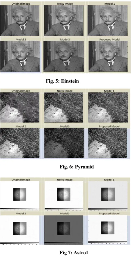
Fig. 5: Einstein

Fig. 6: Pyramid

Fig 7: Astro1

Fig 8: Astro2

7.

CONCLUSION

performance in all the types of images tested with in terms of PSNR and IQI. It is also observed that application of bilateral filters on wavelet decomposed subbands in any combination with wavelet thresholding deteriorates the performance of the model, whereas, application of bilateral filters before or after or on both before and after decomposition enhances the performance. So, the model 19, wherein the bilateral filter is applied before decomposition, is found to be the most consistent. Thus, model 19 is recommended as a well competent model for denoising any type of images. The visual quality for the images like Lena, Barbara, Einstein, Pyramid, Astro1 and Astro2 for the models 1, 2, 3 and the proposed model can be examined from Figs. 3 to 8 respectively.

8.

REFERENCES

[1] Mukesh C. Motwani, Mukesh C. Gadiya, Rakhi C. Motwani, Frederick C. Harris, Jr, “Survey of Image Denoising Techniques”, Proc. of GSPx, Santa Clara Convention Center, Santa Clara, CA, pp. 27-30, 2004.

[2] Ming Zhang, Bahadir Gunturk, “A New Image Denoising Method based on the Bilateral Filter”, ICASSP, IEEE, pp. 929-932, 2008.

[3] H. Guo, J. E. Odegard, M. Lang, R. A. Gopinath, I.W. Selesnick, C. S. Burrus, “Wavelet based Speckle Reduction with Application to SAR based ATD/R”, First International Conference on Image Processing, 1, pp. 75-79, 1994.

[4] Robert D. Nowak, “Wavelet Based Rician Noise Removal”, IEEE Transactions on Image Processing, 8(10), pp. 1408-1419, 1999.

[5] A Chambolle. et al., “Nonlinear Wavelet Image Processing: Variational Problems, Compression, and Noise Removal through Wavelet Shrinkage”, IEEE Trans. Image processing, 7, pp. 319-335, 1998.

[6] K. Egiazarian, et al., “Adaptive Denoising and Lossy Compression of Images in Transform Domain”, Journal of Electronic Imaging, 8(3), pp. 233-245, 1999.

[7] G.L Fan, and X.G. Xia, “Image Denoising Using Local Contextual Hidden Markov Model in the Wavelet Domain”, IEEE Signal Processing Letters, 8(5), pp. 125-128, 2001.

[8] I. Daubechies, “The Wavelet Transform, Time-frequency Localization and Signal Analysis”, IEEE Trans. Inform. Theory, 36, pp. 961-1005, 1990.

[9] S. Mallat, “A Theory for Multiresolution Signal Decomposition: the Wavelet Representation”, IEEE Trans. on Patt. Anal. Mach Intell., pp. 674-693, 1989.

[10]D.L. Donoho, I.M. Johnstone, “Ideal Spatial Adaptation by Wavelet Shrinkage”, Biometrika, 81(3), pp. 425–455, 1994.

[11]D. L. Donoho, “De-noising by Soft Thresholding”, IEEE Trans. on Inform, Theory, 41(3), pp. 613- 627, 1995.

[12]Babak Nasersharif, Ahmad Akbari, “Application of Wavelet Transform and Wavelet Thresholding in Robust Subband Speech Recognition”, 12th European Signal Processing Conferences (EUSIPCO), Vienna, Austria, pp. 345-348, 2004.

[13]P. Perona and J. Malik, “Scale-space and Edge Detection using Anisotropic Diffusion”, IEEE Trans. Pattern Analysis and Machine Intelligence, 12(7), pp. 629–639, 1990.

[14]C. Tomasi and R. Manduchi, “Bilateral Filtering for Gray and Color Images”, Proc. Int. Conf. Computer Vision, pp. 839–846, 1998.

[15]L. I. Rudin, S. Osher, and E. Fatemi, “Nonlinear Total Variation based Noise Removal Algorithms”, Physica D, 60(1-4), pp. 259–268, 1992.

[16]A. Buades, B. Coll, and J. Morel, “Neighborhood Filters and PDE’s”, Numerische Mathematik, 105(1), pp. 1-34, 2006.

[17]D. L. Donoho and I. M. Johnstone, “Adapting to Unknown Smoothness via Wavelet Shrinkage”, Journal of the American Statistical Association, 90(432), pp. 1200–1224, 1995.

[18]D. L. Donoho, I. M. Johnstone, G. Kerkyacharian, D. Picard, “Wavelet Shrinkage: Asymptopia”, Journal of Royal Statistics Society, Series B, 57(2), pp. 301–369, 1995.

[19]S G Chang, et al., “Adaptive Wavelet Thresholding for Image Denoising and Compression”, IEEE Transactions on Image Processing, 9, pp. 1532 –1546, 2000.

[20]S.G. Chang, B. Yu, M. Vetterli, “Spatially Adaptive Wavelet Thresholding with Context Modeling for Image Denoising”, Proc. ICIP, pp. 535-539, 1998.

[21]S. Roy, A. K. Sen, N. Sinha, “VQ-DCT based Image Compression: A New Hybrid Approach”, Assam University Journal of Science and Technology, 5(2), pp. 73-80, 2010.

[22]Zhou Wang, Alan C. Bovik, “A Universal Image Quality Index”, IEEE Signal Processing Letters, 9(3), 2002

[23]G. Schwarz, “Estimating the Dimension of a Model”, Annals of Statistics, 6(2), pp. 461–464, 1978.