Estimation of the Reliability Measures of a Three component System with Human Errors and Common Cause Failures

(1)

Estimation of the Reliability Measures of a Three –

Component System with Human Errors and Common

Cause Failures

B. R. Sreedhar

Assistant Professor Dept. Of Mathematics

Chaitanya Bharathi Institute of Technology

Hyderabad, India

K.Pushpanjali

Professor Department Of Statistics

Sri Krishnadevaraya University Anantapur, A.P., India

G. Y. Sagar

Associate Professor Dept. Of Mathematics

T R R Engineering College, Hyderabad, India.

Y. R. Reddy

Teaching Assistant Department Of Or&Sqc Rayalaseema University,

Kurnool, India

ABSTRACT

The present paper discusses the problem of estimating the reliability measures of a three-component identical system when the system is affected by Common Cause Shock (CCS) failures as well as human errors. The maximum likelihood estimators of the reliability measures like reliability function and mean time between failures of the present model are obtained. The performances of the proposed estimates have been developed in terms of mean square error, using simulated data.

General Terms

Three-component identical system, Reliability measures, Reliability estimates, Maximum likelihood estimation.

Keywords

M L estimation, CCS failures, Human errors, Reliability function, MTBF, Monte-Carlo Simulation.

1. INTRODUCTION

In modern industries very high reliability systems are needed but it is universally accepted that computers cannot achieve the intended reliability in operating systems, application programs, control programs or commercial systems such as space shuttle, nuclear power plant control, etc., without employing redundancy. Further, there are other factors such as Common Cause Shock (CCS) failures and human errors etc. which could cause the whole system to fail. Therefore, the interest lies in assessing and estimating system performance measures like Reliability function, Mean time between failures (MTBF) etc. in the presence of the above said failures. However estimation methods and techniques were available for estimating the parameters and reliability of the system in the literature. Sagar et al [6] derived the reliability measures of a three component identical system with CCS failures and human errors. Billinton and Allan [2] discussed the role of Common cause failures in reliability modeling. Atwood [1] used the BFR model for Common cause failures in the area of nuclear power plants. Chari et al [3] derived the reliability measures of a two component identical system under the influence of CCS failures. Ritika wason [5] studied the traditional software reliability estimation. Reddy [4] derived reliability measures in the presence of lethal and non-lethal CCS failures of a two component non-identical system.

In this paper, we have tried to evaluate the estimation approach which could give formal estimation procedure of the reliability measures with specific reference to CCS failures as well as human errors. In this connection, we considered three-component identical system with CCS failures as well as human errors and the M L estimation approach is proposed to estimate the reliability measures of the present model.

Therefore, the purpose of this paper is not only to estimate the reliability measures but also to report on the results of our simulation study and to resolve differences among other existing studies of system reliability.

2. NOTATIONS

λi, λc & λh : rate of individual, CCS failures and human

errors respectively

p1, p2 & p3 : chance of individual, CCS failures and human

errors respectively µ0 and µ1 : repair rates

) (t chs

R : reliability function for series system with CCS failures as well as human errors

) (

ˆ _t

chs

R : M L estimate of reliability function for series system with CCS failures as well as human errors

) (t chp

R : reliability function for parallel system with CCS failures as well as human errors )

(

ˆ _t

chp

R : M L estimate of reliability function for parallel system with CCS failures as well as human errors

) (T chs

E : expected time of failure for series system (MTTF/MTBF) with CCS failures as well as human errors

) (

ˆ _T

chs

E : M L estimate of expected mean time of failure for series system with CCS failures as well as human errors

) (T chp

E : expected time of failure for parallel system

(MTTF/MTBF) with CCS failures as well as human errors

) (

ˆ _T

chp

E : M L estimate of expected mean time of failure for parallel system with CCS failures as well as human errors

w & y ,

(2)

CCS failures and human errors respectively z : sample mean of service time of the components

wˆ & yˆ ,

xˆ : sample estimates of individual failure rate, CCS failure rate and human errors respectively

zˆ : sample estimate of service time of the components

n : sample size

N : number of simulated samples M S E : mean square error

3. ASSUMPTIONS

(i) The system consists of three s-independent and identical components.

(ii) The system is affected by individual, CCS failures and human errors

(iii) The arrival stream of individual failures, CCS failures and human errors from a Poisson process with arrival rates λi, λc & λh respectively. The

chance of such failures are p1, p2 & p3 such that

p1+p2+p3 = 1.

(iv) The times between individual failures, CCS failures and human errors follow an exponential distribution.

(v) The individual failures, CCS failures and human errors occurs independent of each other.

(vi) The failed components are repaired singly and repair times follow an exponential distribution with rate of repair „µ‟.

4. THE MODEL

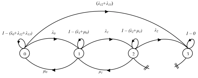
Keeping in view of the above assumptions, we formulate a Markov model to obtain the reliability function and MTBF of the system under the influence of individual, common cause shock failures as well as human errors. The Markovian graph is given in Fig. (4.1) and the quantities appear in Fig. (4.1) are to be read as

λ0 = 3λi p1 ; λ1 = 2λi p1 ; λ2 = λi p1 ; λ12 = λc p2 ; λ13 = λh p3 ;

μ0 = μ ; μ1 = 2μ

The differential equations associated with the system states are

p'0 = – (3λi p1 + λc p2 + λh p3) p0 (t) + p1 (t) μ

p'1 = (3λi p1) p0 (t) – (2λi p1 + μ) p1 (t) + 2μ p2 (t)

p'2 = (2λi p1) p1 (t) – (λi p1 + 2μ) p2 (t)

p'3 = (λc p2 + λh p3) p0 (t) + (λi p1) p2 (t) (1)

Using the Laplace transformation, the set of equations in (1) can be solve with the help of the initial conditions given at t = 0, p0 (t) = 1 and p1 (t) = p2 (t) = p3 (t) = 0 and the solution

is

p0 (t) = [(12 + 1 K + L) / (1 – 2) (1 – 3)] exp (1t)

– [(2 2

+ 2 K + L) / (1 – 2) (2 – 3)] exp (2t)

+ [(32 + 3 K + L) / (1 – 3) (2 – 3)] exp (3t) (2)

p1 (t) = [(3i p1) (1 + i p1 + 2) / (1 – 2) (1 – 3)] exp (1t)

– [(3i p1) (2 + i p1 + 2) / (1 – 2) (2 – 3)] exp (2t)

+[(3i p1) (3 + i p1 + 2) / (1 – 3) (2 – 3)] exp (3t)

(3) p2 (t) = [6(i p1)

2

/ (1 – 2) (1 – 3)] exp (1t)

– [6(i p1)2 / (1 – 2) (2 – 3)] exp (2t)

+[6(i p1)2 / (1 – 3) (2 – 3)] exp (3t) (4)

p3 (t) = 1 – [ p0 (t) + p1 (t) + p2 (t) ] (5)

Where

K = (3i p1 + 3)

L = (2(i p1)2 + i p1  + 22) (6)

1 = –  sin(α) – S1/3

2 = sin (π/3+α) – S1/3

3 = sin (– π/3+α) – S1/3 (7)

Here

= (2/3) (S1 2

–3S2) 1/2

α = sin-1

(– 4q/3)/3 q = S3 – (S1S2)/3 +2 S1

3

/27 and S1, S2 & S3 are defined as follows

S1 = (6i p1 + h p3 + c p2 + 3)

S2 = [11(i p1)2 + 3h p3i p1 + 3cp2i p1 + 7i p1 + 3hp3 + 3cp2 + 2

2

] S3 = [6(i p1)3 + 2(i p1)2 h p3 + 2(i p1)2 c p2

+ 2c p22 + i p1 h p3 + i p1 c p2  + 2h p32 ]

1, 2and 3are always negative ,



i ≥ 0, p1, p2 & p3



(0, 1)

(

λ12+λ13

)

1 – 0

1 – (λ1+μ0) 1 – (λ2+μ1) λ2

1 – (λ0+λ12+λ13)

μ1

μ0 ◄ ◄

► ►

►

0

2

0

1

0

3

[image:2.595.95.515.301.467.2]

λ0 λ1

(3)

5. MAXIMUM LIKELIHOOD (M L)

ESTIMATION OF THE RELIABILITY

MEASURES

This section discusses the Maximum likelihood estimation approach for estimating the reliability measures of three component identical series and parallel systems in the presence of individual, CCS failures as well as human errors.

Let x₁,x₂,...x_n be a sample of „n‟ number of times between individual failures which will obey exponential law.

Let y1,y2,...yn be a sample of „n‟ number of times

between CCS failures which follow exponential as well. Let w₁,w₂,...w_n be a sample of „n‟ number of times between human errors which follow exponential as well.

Let z1,z2,...zn be a sample of „n‟ number of times

repair of the components with exponential population law.

z w y

xˆ,ˆ,ˆ&ˆ are the maximum likelihood estimates of individual failure rate (λi), CCS failure rate (λc), human errors

rate (λh) and repair rate „µ‟ of the system respectively.

Where,

x xˆ1

;

y yˆ1

;

w wˆ 1

;

z zˆ1 and

n x x_ i

_;

n y y_ i

_;

n w w_ i

_;

n z z_ i

are the sample estimates of the rate of individual failure times, rate of CCS failure times, rate of human error times and rate of repair times of the components respectively.

5.1 Estimation of the Reliability function –

Series system

The reliability function for series system is obtained as )

(t chs

R = p0 (t)

=R1 exp (1 t ) – R2 exp (2 t ) + R3 exp (3t) (8)

Where

R1 = ( 12 + 1K + L ) / (1 – 2)( 1 – 3)

R2 = ( 2 2

+ 2K + L ) / (1 – 2)( 2 – 3)

R3 = ( 32 + 3K + L ) / (1 – 3)( 2 – 3)

K, L and 1, 2,3 are given in (6) & (7) respectively.

The reliability expression given in (8) agrees with the result already developed by sagar et al [6]. For series system, we do not consider repairs, i.e µ0 = µ1 = 0 in the model. Therefore, the

successful operation is shown by state „0‟ of the model. By substituting 1, 2 and 3as seen in (8), it can be simplified to

) (t chs

R = exp [– (3λi p1 + λc p2 + λh p3) t ] (9)

Therefore, the maximum likelihood estimation of the reliability function for series system is given by

)) ˆ ˆ ˆ 3 ( exp( ) ( ˆ 3 2 1 yp wp

p x t

Rchs     (10)

Where xˆ,yˆ&wˆare the samples estimates given in “section 5”.

5.2 Estimation of the Reliability function –

Parallel system

The reliability function for parallel system is obtained as

) (t

R_chp = p0 (t) + p1 (t) + p2 (t)

= J1 exp (1 t ) – J2 exp (2 t ) + J3 exp (3t) (11)

Where,

J1 = [(12 + 1K + L) + (3i p1) (1 + i p1 + 2) + 6(i p1)2 ] /

(1 – 2) (1 – 3)

J2 = [(22 + 2 K + L) + (3i p1) (2 + i p1 + 2) + 6(i p1)2 ] /

(1 – 2) (2 – 3)

J3 = [(3 2

+ 3 K + L) + (3i p1) (3 + i p1 + 2) + 6(i p1) 2

] / (1 – 3) (2 – 3)

K, L, and 1,2, 3 are given in (6) and (7) respectively.

The reliability expression given in (11) agrees with the result already developed by Sagar et al [6]. Therefore, the maximum likelihood estimate of the reliability function for parallel system is given by

) exp( ) exp( ) exp( ) ( ˆ 3 ' 3 2 ' 2 1 '

1 Dt J Dt J Dt

J t

R_chp   

(12)

Where,





 

  











 

  











 

  



1 3



2 3



2 1 1 3 1 1 ' 3 2 3 ' 3 3 2 2 1 2 1 1 2 1 1 ' 2 2 2 ' 2 3 1 2 1 2 1 1 1 1 1 ' 1 2 1 ' 1 ˆ 6 ˆ 2 ˆ ˆ 3 ˆ 6 ˆ 2 ˆ ˆ 3 ˆ 6 ˆ 2 ˆ ˆ 3 D D D D p x z p x D p x L K D D J D D D D p x z p x D p x L K D D J D D D D p x z p x D p x L K D D J       _ _ _ _ _ _        _ _ _ _ _ _        _ _ _ _ _ _ 





 

2 1 2 1 ' 1 ' ˆ 2 ˆ ˆ ˆ 2 ˆ 3 ˆ 3 z z p x p x L z p x K     

(13)

 







/3



/3 sin 3 / 3 / sin 3 / sin ' 1 ' 3 ' 1 ' 2 ' 1 ' 1 S D D S D D S D D               

(14)

Where,

 

1/2

' 2 2 ' 1 3 3 / 2       _

 S S

D







sin1 4 '/ 3



3

' D q    

 

3 2

 

1'3 27

' 2 ' 1 ' 3 ' S S S S

q   



xp wp yp z



S₁'6ˆ ₁ˆ ₃ˆ ₂3ˆ

 

_

 

 _ _ _ _ _ _

 1 3 1 2 1 3 2 2

2 1 '

2 11xˆp 3xˆpwˆp 3xˆpyˆp 7xˆpzˆ 3wˆpzˆ 3yˆpzˆ 2ˆz

S

            

          

               2 3 2 1 3 1 2 2 2 2 1 3 2 1 3 1 ' 3 ˆ ˆ 2 ˆ ˆ ˆ ˆ ˆ ˆ ˆ ˆ 2 ˆ ˆ 2 ˆ ˆ 2 ˆ 6 z p w z p y p x z p w p x z p y p y p x p w p x p x S

(4)

5.3 Estimation of the MTBF function –

Series system

The mean time between failure function for series system is obtain as







0

).

(

)

(

T

R

t

dt

E

_chs _chs

Using the result in (9), the expression reduces to

) (T chs

E = 1 / (3λi p1 + λc p2 + λh p3) (15)

The above expression given in (15) agrees with the result already developed by Sagar et al [6]. Therefore, the maximum likelihood estimate of mean time between failures function for series system is given by



3 ˆ

1

ˆ

2

ˆ

3



1 )

(

ˆ

p

w

p

y

p

x

T

E

_chs





₍₁₆₎

Where xˆ,yˆ&wˆare sample estimates given in “section 5”.

5.4 Estimation of the MTBF function –

Parallel system

The mean time between failure function for parallel system is obtained as







0

).

(

)

(

T

R

t

dt

E

_chp _chp

Using the result in (11), the expression reduces to

)

(

T

E

_chp = – [(6i p1µ + 9(i p1)2 + L) /(1 2 3 )] (17)

Where L and 1 2 3 are given in (6) & (7) respectively.

The above expression given in (17) agrees with the result already developed by Sagar et al [6]. Therefore, the maximum likelihood estimate of mean time between failure function for parallel system is given by

 



1 2 3



' 2 1 1

ˆ

9 ˆ

ˆ

6 )

(

ˆ

D

L

p

x

z

p

x

T

E

_chp













_





(18)

Where L' and D1, D2, D3 are given in (13) and (14)

respectively.

6. SIMULATION STUDY

In the present work, the M L estimates of reliability and MTBF (both series and parallel systems) were not identified with exact or analytical form of probability density function since they are complex functions of sample information. Hence an attempt is made to develop empirical evidence of M L estimation approach by Monte-Carlo Simulation using an appropriate computer package for validity of results.

For a range of specified values of the rates of individual (λi),

CCS failures (λc), human errors (λh) and service rate (µ) and

for the samples of sizes n=5(5)30 were simulated in each case

with N=10,000(20,000)90,000 in order to evolve Mean Square Error (MSE) in each case. For large samples M L estimators are undisputedly better since they are CAN estimators. Interestingly, our simulation study shows that the M L estimate is still reasonably good giving near accurate estimate even for a sample size as low as five (i.e n=5). This shows that M L approach and estimators are quite useful in estimating reliability indices.

[image:4.595.319.540.255.595.2]

6.1 Numerical Illustration

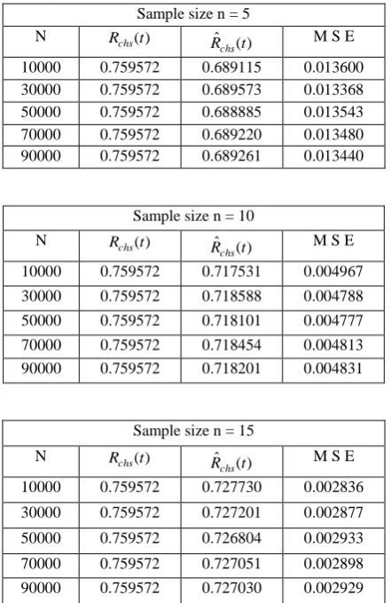
Table 6.1

Reliability function for three component identical Series system with i = 0.1; c = 0.2; h = 0.3; p1 = 0.5; p2 = 0.25;

p3 = 0.25; t = 1

Sample size n = 5

N R_chs(t) _Rˆ ₍_t₎

chs M S E

10000 0.759572 0.689115 0.013600

30000 0.759572 0.689573 0.013368

50000 0.759572 0.688885 0.013543

70000 0.759572 0.689220 0.013480

90000 0.759572 0.689261 0.013440

Sample size n = 10 N Rchs(t) _Rˆ ₍_t₎

chs M S E

10000 0.759572 0.717531 0.004967

30000 0.759572 0.718588 0.004788

50000 0.759572 0.718101 0.004777

70000 0.759572 0.718454 0.004813

90000 0.759572 0.718201 0.004831

Sample size n = 15

chs M S E

10000 0.759572 0.727730 0.002836

30000 0.759572 0.727201 0.002877

50000 0.759572 0.726804 0.002933

70000 0.759572 0.727051 0.002898

90000 0.759572 0.727030 0.002929

Sample size n = 20

N Rchs(t) Rˆ_chs(t) M S E

10000 0.759572 0.731413 0.002082

30000 0.759572 0.731192 0.002126

50000 0.759572 0.731460 0.002097

70000 0.759572 0.731542 0.002108

(5)

Sample size n = 25

chs

M S E

10000 0.759572 0.733631 0.001708

30000 0.759572 0.733851 0.001673

50000 0.759572 0.733953 0.001668

70000 0.759572 0.733852 0.001677

90000 0.759572 0.733986 0.001664

Sample size n = 30

chs M S E

10000 0.759572 0.735627 0.001394

30000 0.759572 0.735225 0.001419

50000 0.759572 0.735542 0.001399

70000 0.759572 0.735537 0.001404

90000 0.759572 0.735497 0.001410

Table 6.2

Reliability function for three component identical Parallel system with i = 0.1; c = 0.2; h = 0.3; p1 = 0.5; p2 = 0.25;

p3 = 0.25; µ = 0.5; t = 1

Sample size n = 5

N R_chp(t) _Rˆ ₍_t₎

chp

M S E

10000 0.887175 0.849740 0.004932

30000 0.887175 0.850022 0.004915

50000 0.887175 0.850103 0.004870

70000 0.887175 0.850430 0.004762

90000 0.887175 0.849990 0.004864

Sample size n = 10

N R_chp(t) _Rˆ ₍_t₎

chp M S E

10000 0.887175 0.865974 0.001597

30000 0.887175 0.865919 0.001601

50000 0.887175 0.865943 0.001606

70000 0.887175 0.865985 0.001584

90000 0.887175 0.865867 0.001597

Sample size n = 15

N Rchp(t) Rˆ_chp(t) M S E

10000 0.887175 0.870512 0.000914

30000 0.887175 0.870614 0.000928

50000 0.887175 0.870613 0.000941

70000 0.887175 0.870641 0.000932

90000 0.887175 0.870702 0.000934

Sample size n = 20

N Rchp(t) _Rˆ ₍_t₎

chp M S E

10000 0.887175 0.873056 0.000657

30000 0.887175 0.873026 0.000662

50000 0.887175 0.872856 0.000667

70000 0.887175 0.872931 0.000667

90000 0.887175 0.872983 0.000655

Sample size n = 25

chp M S E

10000 0.887175 0.874175 0.000522

30000 0.887175 0.874230 0.000523

50000 0.887175 0.874086 0.000527

70000 0.887175 0.874210 0.000521

90000 0.887175 0.874168 0.000519

Sample size n = 30

chp M S E

10000 0.887175 0.875058 0.000436

30000 0.887175 0.875115 0.000430

50000 0.887175 0.875075 0.000435

70000 0.887175 0.874990 0.000438

[image:5.595.319.538.68.428.2]

90000 0.887175 0.874957 0.000438

Table 6.3

Simulation results for Mean Time Between Failures function Series System with i = 0.5; c = 0.6; h = 0.7; p1 = 0.5;

p2 = 0.25; p3 = 0.25

Sample size n = 5

N Echs(T) Eˆ_chs(T) M S E

10000 0.930233 0.775375 0.100702

30000 0.930233 0.774135 0.098398

50000 0.930233 0.772012 0.099046

70000 0.930233 0.773719 0.099438

90000 0.930233 0.773195 0.099385

Sample size n = 10

N E_chs(T) _Eˆ ₍_T₎

chs

M S E

10000 0.930233 0.815011 0.053551

30000 0.930233 0.818934 0.053011

50000 0.930233 0.817060 0.052856

70000 0.930233 0.818580 0.053243

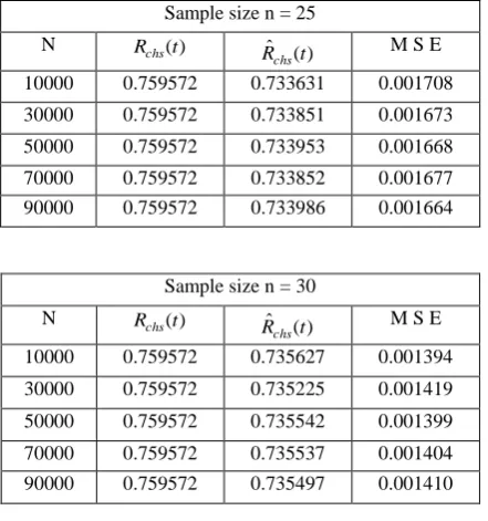
[image:5.595.58.279.72.308.2]

(6)

Sample size n = 15

10000 0.930233 0.835785 0.036667

30000 0.930233 0.833126 0.037403

50000 0.930233 0.831677 0.037694

70000 0.930233 0.832914 0.037361

90000 0.930233 0.832948 0.037576

Sample size n = 20

10000 0.930233 0.839737 0.029085

30000 0.930233 0.840229 0.029468

50000 0.930233 0.840799 0.029124

70000 0.930233 0.841224 0.029375

90000 0.930233 0.840687 0.029251

Sample size n = 25

10000 0.930233 0.843980 0.024777

30000 0.930233 0.844510 0.024431

50000 0.930233 0.845286 0.024315

70000 0.930233 0.844804 0.024478

90000 0.930233 0.845343 0.024297

Sample size n = 30

10000 0.930233 0.848411 0.021064

30000 0.930233 0.846535 0.021355

50000 0.930233 0.848110 0.021092

70000 0.930233 0.847995 0.021174

[image:6.595.55.278.71.544.2]

90000 0.930233 0.847722 0.021248

Table 6.4

Simulation results for Mean Time Between Failures function Parallel System with i = 0.5; c = 1.5; h = 2; p1 = 0.5;

p2 = 0.25; p3 = 0.25; µ= 5

Sample size n = 5

N E_chp(T) _Eˆ ₍_T₎

chp M S E

10000 1.169361 1.020356 0.178590

30000 1.169361 1.024095 0.180666

50000 1.169361 1.021380 0.179231

70000 1.169361 1.023405 0.178946

90000 1.169361 1.021091 0.180232

Sample size n = 10

chp M S E

10000 1.169361 1.052237 0.093493

30000 1.169361 1.050642 0.093152

50000 1.169361 1.051699 0.093652

70000 1.169361 1.051567 0.093196

90000 1.169361 1.050292 0.093135

Sample size n = 15

N Echp(T) Eˆ_chp(T) M S E

10000 1.169361 1.059674 0.063832

30000 1.169361 1.060975 0.063887

50000 1.169361 1.061927 0.064016

70000 1.169361 1.061602 0.064046

90000 1.169361 1.062657 0.064234

Sample size n = 20

chp M S E

10000 1.169361 1.069577 0.049401

30000 1.169361 1.068467 0.049425

50000 1.169361 1.067072 0.049651

70000 1.169361 1.067911 0.049747

90000 1.169361 1.068214 0.049237

Sample size n = 25

N Echp(T) Eˆ_chp(T) M S E

10000 1.169361 1.070323 0.040910

30000 1.169361 1.070973 0.041083

50000 1.169361 1.069865 0.041186

70000 1.169361 1.070826 0.040923

90000 1.169361 1.070431 0.040869

Sample size n = 30

chp M S E

10000 1.169361 1.072988 0.035464

30000 1.169361 1.073722 0.035274

50000 1.169361 1.073574 0.035206

70000 1.169361 1.072761 0.035357

90000 1.169361 1.072214 0.035439

7. CONCLUSIONS

(7)

square error is almost zero with sample sizes „n‟ tending to large i.e 20 and above.

Therefore, the M L estimators are generally hard to beat consistently, even in small samples and our simulation results showed a strong preference for the M L estimation method for situations arising in practical reliability analysis.

8. REFERENCES

[1] Atwood, C. L. (1986) “The binomial failure rate common cause model” in Technometrics, vol: 28, pp. 139-147.

[2] Billinton, R & Allan, R. N (1983) “Reliability Evaluation of Engineering Systems; Concepts and Techniques”, Plenum Press, New York.

[3] Chari, A. A., Sastry, M. P and Madhusudhana Verma, S. (1991) “Reliability analysis in the presence of common

cause shock failures”, Micro-Electronics and reliability,31, pp.15-19.

[4] Reddy, Y. R. (2003) “Reliability analysis for two unit non-identical system with CCS failures”, Ph.D thesis, S.K.University, Anantapur.

[5] Ritika Wason, Ahmed. P and Qasim Rafiq, M. (2012), “New paradigm for software reliability estimation”, International journal of computer application, vol.44, No.14, pp. 39-44.