The Solution of Nonlinear Equations via the Method of Hurwitz Radon Matrices

(1)

http://dx.doi.org/10.4236/jcc.2014.210002

The Solution of Nonlinear Equations via the

Method of Hurwitz-Radon Matrices

Dariusz Jacek Jakóbczak

Department of Electronics and Computer Science, Technical University of Koszalin, Koszalin, Poland Email: [email protected]

Received 11 May 2014; revised 10 June 2014; accepted 5 July 2014

This work is licensed under the Creative Commons Attribution International License (CC BY). http://creativecommons.org/licenses/by/4.0/

Abstract

Image analysis and computer vision are interested in suitable methods to solve the nonlinear eq-uations. Coordinate x for f x

( )

=0 is crucial because each equation can be transformed into

( )

0

f x = . A novel method of Hurwitz-Radon Matrices (MHR) can be used in approximation of a

root of function in the plane. The paper contains a way of data approximation via MHR method to solve any equation. Proposed method is based on the family of Hurwitz-Radon (HR) matrices. The matrices are skew-symmetric and possess columns composed of orthogonal vectors. The operator of Hurwitz-Radon (OHR), built from these matrices, is described. Two-dimensional data are re- presented by discrete set of curve f points. It is shown how to create the orthogonal OHR oper-ator and how to use it in a process of data interpolation. MHR method is interpolating the curve point by point without using any formula or function.

Keywords

Image Analysis, Nonlinear Equation, Root of Function, Curve Interpolation, Hurwitz-Radon Matrices

1. Introduction

A significant problem in computer vision and image analysis [1] is to solve any nonlinear equation

( )

(2)

exam-ple in Newton’s method we may find difficulties in calculating derivative of a function or troubles with bad starting point of iteration. Generally iterative methods need many assumptions about function (monotonicity, convexity, derivative, starting point). Some methods are used only for polynomials (Muller’s, Laguerre’s, Bair- stow’s, Jenkins-Traub’s methods). Nonlinear systems are still opened for researchers [3].

This paper is dealing with novel method of root’s approximation by using a family of Hurwitz-Radon matric-es. Method of Hurwitz-Radon Matrices (MHR) does not need any assumption about function. The only informa-tion about curve is the set of at least five interpolainforma-tion nodes and a zero of the funcinforma-tion between two of them. Proposed method of Hurwitz-Radon Matrices (MHR) is used in data interpolation and then calculations to solve the nonlinear equation are introduced. MHR connects two significant problems in mathematics and computer sciences: interpolation of the function and the solution of nonlinear equation [4]. MHR method uses two-dimensional data for knowledge representation [5] and computational foundations [6]. Also medicine [7], industry and manufacturing are looking for the methods connected with geometry of the curves [8]. So suitable data re-presentation and precise solving of any equation [9] are the key factors in many applications of artificial intelli-gence and numerical methods [10].

2. Assumptions for the Solution

Each nonlinear equation is represented by f x

( )

=0 and succeeding points

(

x y_i, _i

)

∈R2 of function f (in-terpolation nodes) as follows in proposed MHR method:

1. first node

(

x y₁, ₁

)

and last node

(

x_L,y_L

)

must fulfill a condition y₁⋅yL <0;

2. at least three nodes

(

x y₂, ₂

) (

, x y₃, ₃

) (

, x y₄, ₄

)

, for example equidistant between first and last node, have to be calculated (for L=5) if MHR method is used with matrices of dimension N=2.

[image:2.595.135.498.561.703.2]

Condition 1 is well known in numerical methods for existing a zero of the function. Condition 2 is connected with important features of MHR method: MHR version with matrices of dimension N=2 (called MHR-2) needs at least five nodes (for L=5), MHR version with matrices of dimension N=4 (called MHR-4) needs at least nine nodes (for L=9) and MHR version with matrices of dimension N=8 (called MHR-8) needs at least 17 nodes (for L=17).

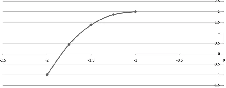
Figure 1 presents the graph of function f x

( )

=x3+x2− +x 1 with nodes: first

(

− −2; 1 ,

) (

−1.75; 0.453125 ,

)

(

−1.5;1.375 ,

) (

−1.25;1.859375

)

and last

(

−1; 2

)

. All five nodes are applied in MHR calculations, but a root of function is searched only between nodes

(

− −2; 1

)

and

(

−1.75; 0.453125

)

. The approximation of a zero point of the function is possible using novel MHR method.

3. Reconstruction of the Graph Points

The key question exists in many branches of science: is it possible to find a method of nonlinear equation solu-tion without iterasolu-tions of numerical methods [11]? This paper aims at giving the positive answer to this question. Method of Hurwitz-Radon Matrices (MHR), described in this paper, is computing points between two succes-sive nodes for searching a root of the function. The curve or function in MHR method is parameterized for real number α∈

[ ]

0;1 in the range of two successive interpolation nodes.

Figure 1.Five nodes of function and a root between first and second node (MS Excel graph).

-1.5 -1 -0.5 0 0.5 1 1.5 2 2.5

(3)

3.1. The Operator of Hurwitz-Radon

Adolf Hurwitz (1859-1919) and Johann Radon (1887-1956) published the papers about specific class of matric-es in 1923, working on the problem of quadratic forms. Matricmatric-es A_i, i=1, 2,m satisfying

2

0, for ; , 1, 2, ,

j k k j j

A A +A A = A = −I j≠k j k=  m

are called a family of Hurwitz-Radon matrices. A family of Hurwitz-Radon (HR) matrices has important fea-tures [12]: HR matrices are skew-symmetric

(

A_iT = −A_i

)

and reverse matrices are easy to find

(

A_i−1= −A_i

)

. Only for dimension N =2, 4 or 8 the family of HR matrices consists of N−1 matrices. For N=2 there is one matrix: 1 0 1 . 1 0   = ₋    A

For N=4 there are three HR matrices with integer entries:

1 2 3

0 1 0 0 0 0 1 0 0 0 0 1

1 0 0 0 0 0 0 1 0 0 1 0

, , .

0 0 0 1 1 0 0 0 0 1 0 0

0 0 1 0 0 1 0 0 1 0 0 0

      ₋     ₋        =_ _ =_ _ =_ _ − −    ₋  ₋       

A A A

For N=8 we have seven HR matrices with elements 0, ±1. So far HR matrices are applied in electronics [13]: in Space-Time Block Coding (STBC) and orthogonal design [14], also in signal processing [15] and Ha-miltonian Neural Nets [16].

If one curve is described by a set of following points

{

(

x yi, i

)

,i=1, 2,,n

}

then HR matrices combined

with the identity matrix IN are used to build the orthogonal and discrete Hurwitz-Radon Operator (OHR). For nodes

(

x y₁, ₁

)

and

(

x y₂, ₂

)

OHR M of dimension N=2 is constructed:

1 1 2 2 2 1 1 2 2 2

1 2 2 1 1 1 2 2 1 2

1 x y x y x y x y M

x y x y x y x y

x x

+ −

 

= _ _

− +

+ _ _. (1)

For nodes

(

x y₁, ₁

) (

, x y₂, ₂

) (

, x y₃, ₃

)

and

(

x y₄, ₄

)

OHR of dimension N=4 is constructed:

0 1 2 3

1 0 3 2

2 2 2 2

2 3 0 1

1 2 3 4

3 2 1 0

1

u u u u

M

u u u u

x x x x

u u u u

  ₋ ₋    = − −  + + + ₋ ₋    (2) where

0 1 1 2 2 3 3 4 4 1 1 2 2 1 3 4 4 3

2 1 3 2 4 3 1 4 2 3 1 4 2 3 3 2 4 1

, ,

, .

u x y x y x y x y u x y x y x y x y

= + + + = − + + −

= − − + + = − + − +

For nodes

(

x y₁, ₁

) (

, x y₂, ₂

)

, and

(

x y₈, ₈

)

OHR of dimension N=8 is built [17] similarly as (1) and

(2):

0 1 2 3 4 5 6 7

1 0 3 2 5 4 7 6

2 3 0 1 6 7 4 5

3 2 1 0 7 6 5 4

8

2 4 5 6 7 0 1 2 3

1 ₅ ₄ ₇ ₆ ₁ ₀ ₃ ₂

6 7 4 5 2 3 0 1

7 6 5 4 3 2 1 0

1

i i

u u u u u u u u

M

u u u u u u u u

x

u u u u u u u u

=   ₋ ₋ ₋ ₋    − − − −  ₋ ₋ ₋ ₋    = _ _ − − − −   − − − −   ₋ ₋ ₋ ₋    − − − −    

(4)

where

1 2 3 4 5 6 7 8 1

2 1 4 3 6 5 8 7 2

3 4 1 2 7 8 5 6 3

4 3 2 1 8 7 6 5 4

5 6 7 8 1 2 3 4 5

6 5 8 7 2 1 4 3 6

7 8 5 6 3 4 1 2 7

8 7 6 5 4 3 2 1

y y y y y y y y x

u

y y y y y y y y x

  ₋ ₋ ₋ ₋    − − − −  ₋ ₋ ₋ ₋    =_ _⋅ − − − −   − − − −   ₋ ₋ ₋ ₋    − − − −  

  8

                          (4)

The components of the vector u=

(

u u₀, ,₁,u₇

)

T, appearing in the matrix M (3), are defined by (4) in the similar way to (1) and (2) but in terms of the coordinates of the above 8 nodes. Note that OHR operators M (1)-(3) satisfy the condition of interpolation

M⋅ =x y (5)

For x=

(

x x₁, ₂,,xN

)

T∈RN,x≠0, y=

(

y y₁, ₂,,yN

)

T∈RN,N =2, 4 or 8.

3.2. Points Interpolation by MHR

Key question looks as follows: how can we compute coordinates of points settled between the interpolation nodes [18]? The answer is connected with novel MHR method [19]. On a segment of a line every number “c” situated between “a” and “b” is described by a linear (convex) combination c= ⋅ + −α a

(

1 α

)

⋅b for

[ ]

0;1 . b c

b a

α= − ∈

− (6)

The average OHR operator M₂ of dimension N =2, 4 or 8 is constructed as follows:

(

)

2 0 1 1

M = ⋅α M + −α ⋅M (7)

with the operator M₀ built (1)-(3) by “odd” nodes

(

x₁=a y, ₁

) (

, x y₃, ₃

)

,,

(

x₂_N₋₁,y₂_N₋₁

)

and M₁ built (1)-(3) by “even” nodes

(

x₂ =b y, ₂

) (

, x y₄, ₄

)

,,

(

x₂_N,y₂_N

)

. Having the operator M₂ it is possible to reconstruct the second coordinates of points

( )

x y, in terms of the vector C defined with

(

)

2 1 1 2, 1, 2, ,

i i i

c = ⋅α x ₋ + −α ⋅x i=  N (8)

as C=

[

c c₁, ₂,,cN

]

T. The required formula is similar to (5):

( )

2

Y C =M ⋅C (9)

in which components of vector Y C

( )

give the second coordinate of the points

( )

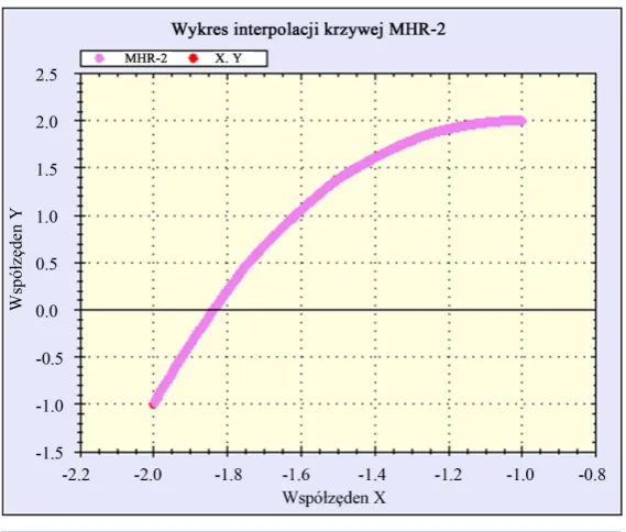
x y, corresponding to the first coordinate, given in terms of components of the vector C.

Calculations of unknown coordinates for curve points using (6)-(9) are called by author the method of Hur-witz-Radon Matrices (MHR) [20]. Here is the application of MHR method (Figure 2) for function

( )

3 2

1

f x =x +x − +x with nodes as Figure 1and computed 99 points between each pair of nodes

(

α =0.01, 0.02,, 0.99

)

.

Solving the equation x3+x2− + =x 1 0 via MHR interpolation, as it was said under Figure 1, we search a root of the function only between nodes

(

− −2; 1

)

and

(

−1.75; 0.453125

)

. Points calculated between other pairs of nodes are useless in the process of root approximation and they don’t have to be computed. Considering calculated points between nodes

(

− −2; 1

)

and

(

−1.75; 0.453125

)

, second coordinate is near zero at

(

−1.835; 0.00184

)

. Solution of equation x3+x2− + =x 1 0 via MHR-2 method is approximated by

1.835

x= − . True value is x= −1.839.

(5)

[image:5.595.171.456.82.324.2]

Figure 2.Function

( )

3 2

1

f x =x +x − +x with 396 interpolated points using MHR-2 method.

very important feature.

4. Nonlinear Equations Solved via MHR

Example 1

MHR calculations are done for function f x

( )

=x3+ln 7

(

−x

)

with nodes:

(

− −2; 5.803 ,

) (

−1.75; 3.190 ,−

) (

−1.5; 1.235 ,−

) (

−1.25; 0.1571

)

and

(

−1;1.0794

)

. So a root of this function is si-tuated between 3rd and 4th node. MHR-2 interpolation gives the graph of function (Figure 3):

Considering points between nodes

(

−1.5; 1.235−

)

and 1.25; 0.1571

(

−

)

, coordinate y is near zero at

(

−1.2825; 0.00194

)

. Solution of equation x3+ln 7

(

−x

)

=0 via MHR method is approximated by

1.2825

x= − . True value is hardly approximated (even for MathCad) by x= −1.28347. Example 2

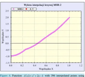
MHR calculations are completed for function

( )

3

2 1

f x =x + x− with nodes:

(

0; 1 , 0.25; 0.484 , 0.5; 0.125 , 0.75; 0.9219−

) (

−

) (

)

and 1; 2 . So a zero of this function is situated between 2

( )

nd and 3rd node. MHR-2 computes the graph of function (Figure 4).

(

0.25; 0.484−

)

and

(

0.5; 0.125 , coordinate y is near zero at

)

(

0.4625; 0.00219 . Solution of equation

)

x3+2x− =1 0 via MHR-2 is approximated by x=0.4625. The only one real solution of this equation is x=0.453.

Now MHR calculations are done for the same equation x3+2x− =1 0 with seven nodes between

(

0; 1−

)

and

( )

1; 2 for xi =0; 0.125; 0.25; 0.375; 0.5; 0.625; 0.75; 0.875 and 1. The solution is approximated by

MHR-4 method with nine nodes. MHR-4 interpolation gives the graph of function (Figure 5).

Considering points between nodes 0.375; 0.197

(

−

)

and

(

0.5; 0.125 , coordinate y is near zero at

)

(

0.45625; 0.00018 . Solution of equation

)

x3+2x− =1 0 via MHR-4 is approximated by x=0.45625. This is better result than MHR-2: greater number of nodes (with the same distance between first and last) means better approximation. And seventeen nodes in MHR-8 guarantee more precise results then MHR-4.

Example 3

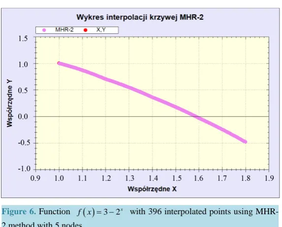
MHR calculations are done for equation 3 2− x =0_{with nodes:}

( ) (

_{1;1 , 1.2; 0.7026 , 1.4; 0.361 , 1.6; 0.031}

) (

₋

)

and

(

1.8; 0.482−

)

. MHR-2 gives the graph of function (Figure 6).

(

1.4; 0.361 and

)

(

1.6; 0.031−

)

, second coordinate is near zero at

(

1.586; 0.000311−

)

. Solution of equation 3 2₋ x ₌0_{via MHR-2 method is approximated by}

1.586

(6)

[image:6.595.171.455.85.286.2]

( )

3

(

)

ln 7

f x =x + −x with 396 interpolated points using MHR-2.

Figure 4. Function

( )

3

2 1

f x =x + x− with 396 interpolated points using MHR-2.

cise solution x=log 3₂ is approximated by 1.585.

Interpolated values, calculated by MHR method, are applied in the process of solving the nonlinear equations. Shorter distance between first and last node or greater number of nodes guarantee better approximation. Ap-proximated solutions of nonlinear equations are used in many branches of computer sciences. MHR joins two important problems: interpolation of the function with the solution of nonlinear equation.

5. Conclusions

[image:6.595.172.456.321.576.2]

(7)

[image:7.595.172.456.86.281.2]

( )

3

2 1

[image:7.595.170.457.316.547.2]

f x =x + x− with interpolated points using MHR- 4 method with 9 nodes.

( )

3 2x

f x = − with 396 interpolated points using MHR- 2 method with 5 nodes.

in MHR method: polynomial or not, monotonicity, convexity, derivative, starting point. These features are very significant for iterative numerical methods. MHR method gives the possibility of reconstruction a curve and searching for a root of the function. The only condition is to have a set of nodes according to assumptions in MHR method. The features of MHR method: accuracy of the equation solution depends on the number of nodes and the distance between first and last node (MHR-4 is more precise than MHR-2 and MHR-8 is more precise than MHR-4); interpolation of a curve consists of L points is connected with the computational cost of rank

( )

O L ; MHR is a well-conditioned method (orthogonal matrices); MHR is not an affine interpolation [22]. Future works are connected with: computing the interpolation error, implementation of MHR in object recog-nition [23], MHR extrapolation method [24] and curve parameterization [25].

References

[1] Ballard, D.H. (1982) Computer Vision. Prentice Hall, New York.

(8)

& Sons, New York. http://dx.doi.org/10.1002/0471705195

[3] Khalil, H.K. (2001) Nonlinear Systems. Prentice Hall, New York.

[4] Kelley, C.T. (1995) Iterative Methods for Linear and Nonlinear Equations. Society for Industrial and Applied Mathe-matics, Philadelphia. http://dx.doi.org/10.1137/1.9781611970944

[5] Markman, A.B. (1998) Knowledge Representation. Lawrence Erlbaum Associates, Mahwah.

[6] Sowa, J.F. (2000) Knowledge Representation: Logical, Philosophical and Computational Foundations. Brooks/Cole, New York.

[7] Soussen, C. and Mohammad-Djafari, A. (2004) Polygonal and Polyhedral Contour Reconstruction in Computed To- mography. IEEE Transactions on Image Processing, 11,1507-1523. http://dx.doi.org/10.1109/TIP.2004.836159

[8] Tang, K. (2005) Geometric Optimization Algorithms in Manufacturing. Computer-Aided Design & Applications, 2, 747-757. http://dx.doi.org/10.1080/16864360.2005.10738338

[9] Kozera, R. (2004) Curve Modeling via Interpolation Based on Multidimensional Reduced Data. Silesian University of Technology Press, Gliwice.

[10] Dahlquist, G. and Bjoerck, A. (1974) Numerical Methods. Prentice Hall, New York.

[11] Ralston, A. (1965) A First Course in Numerical Analysis. McGraw-Hill Book Company, New York.

[12] Eckmann, B. (1999) Topology, Algebra, Analysis-Relations and Missing Links. Notices of the American Mathematical Society, 5, 520-527.

[13] Citko, W., Jakóbczak, D. and Sieńko, W. (2005) On Hurwitz-Radon Matrices Based Signal Processing. Workshop Sig- nal Processing at Poznan University of Technology, Poznan.

[14] Tarokh, V., Jafarkhani, H. and Calderbank, R. (1999) Space-Time Block Codes from Orthogonal Designs. IEEE Transac- tions on Information Theory, 5, 1456-1467. http://dx.doi.org/10.1109/18.771146

[15] Sieńko, W., Citko, W. and Wilamowski, B. (2002) Hamiltonian Neural Nets as a Universal Signal Processor. 28th An-nual Conference of the IEEE Industrial Electronics Society IECON, Sevilla.

[16] Sieńko, W. and Citko, W. (2002) Hamiltonian Neural Net Based Signal Processing. The International Conference on Signal and Electronic System ICSES, Wroclaw.

[17] Jakóbczak, D. (2007) 2D and 3D Image Modeling Using Hurwitz-Radon Matrices. Polish Journal of Environmental Studies, 16, 104-107.

[18] Jakóbczak, D. (2010) Shape Representation and Shape Coefficients via Method of Hurwitz-Radon Matrices. In: Com-puter Vision and Graphics, in: Lecture Notes in Computer Science, 6374, 411-419.

[19] Jakóbczak, D. (2009) Curve Interpolation Using Hurwitz-Radon Matrices. Polish Journal of Environmental Studies, 18, 126-130.

[20] Jakóbczak, D. (2010) Application of Hurwitz-Radon Matrices in Shape Representation. In: Banaszak, Z. and Świć, A., Eds., Applied Computer Science: Modelling of Production Processes, Lublin University of Technology Press, Lublin, 63-74.

[21] Jakóbczak, D. (2010) Object Modeling Using Method of Hurwitz-Radon Matrices of Rank k. In: Wolski, W. and Bo-rawski, M., Eds., Computer Graphics: Selected Issues, University of Szczecin Press, Szczecin, 79-90.

[22] Jakóbczak, D. (2010) Implementation of Hurwitz-Radon Matrices in Shape Representation. In: Choraś, R.S., Ed., Ad-vances in Intelligent and Soft Computing, Vol. 84, Image Processing and CommunicationsChallenges, 39-50. [23] Jakóbczak, D. (2011) Object Recognition via Contour Points Reconstruction Using Hurwitz-Radon Matrices. In: Jó-

zefczyk, J. and Orski, D., Eds., Knowledge-Based Intelligent System Advancements: Systemic and Cybernetic Ap-proaches, IGI Global, Hershey, 87-107.

[24] Jakóbczak, D. (2011) Data Extrapolation and Decision Making via Method of Hurwitz-Radon Matrices. In:Jędrze- jowicz, P., Thanh Nguyen, N. and Hoang, K., Eds., Computational Collective Intelligence, Technologies and Applica-tions, Lecture Notes in Computer Science, Vol. 6922, 173-182.

(9)