Software Reliability Prediction using Neural Network with Encoded Input

Software Reliability Prediction using Neural

Network with Encoded Input

Manjubala Bisi

Reliability Engineering Centre

IIT Kharagpur West Bengal, India

Neeraj Kumar Goyal

Reliability Engineering Centre

IIT Kharagpur West Bengal, India

ABSTRACT

A neural network based software reliability model to predict the cumulative number of failures based on Feed Forward architecture is proposed in this paper. Depending upon the available software failure count data, the execution time is encoded using Exponential and Logarithmic function in order to provide the encoded value as the input to the neural network. The effect of encoding and the effect of different encoding parameter on prediction accuracy have been studied. The effect of architecture of the neural network in terms of hidden nodes has also been studied. The performance of the proposed approach has been tested using eighteen software failure data sets. Numerical results show that the proposed approach is giving acceptable results across different software projects. The performance of the approach has been compared with some statistical models and statistical models with change point considering three datasets. The comparison results show that the proposed model has a good prediction capability.

General Terms

Software reliability prediction, fault count prediction, neural network modeling.

Keywords

Failure prediction, neural network, encoded input, encoded parameter.

1.

INTRODUCTION

In today’s society, many commercial and government organizations use software projects in order to increase their efficiency and effectiveness. Software exists starting from a simple system like mobile to high complex and safety critical system like, air traffic control. As the use of software is increasing, the failures are also increasing rapidly. The consequences of failures may lead to loss of life or economic loss. So, the software professionals need to develop software systems which are not only functionally attractive but also safe and reliable. Software reliability is defined as the probability of failure-free operation of a computer program in a specified environment for a specified time. Reliability of software is measured in terms of failures which are a departure of program operation from program requirements. The software reliability is characterized as a function of failures experienced. Software reliability models are used to describe failures as a random process.

Software engineers can measure or forecast software reliability using software reliability models. In real software development process, cost and time are limited. The models are used to develop reliable software under given time and cost constraints. The software managers also determine the release time of the software with the help these models. In past few years, a large number of software reliability models/statistical models have been developed. Every model

is based on certain assumptions. So the predictive capability of different models is different for different data sets. There exist no single models that can best suit for all cases. The statistical models are also influenced by different external parameters. To overcome these problems, non-parametric models like neural network and support vector machines have been used for last few years. The non-parametric models are not influenced by any external parameter and also not based on assumptions which are unrealistic in real situation. Neural network has become an alternative method in software reliability modeling, evaluation and prediction.

In the literature, many neural network based software reliability prediction models exist and their prediction capability is proven better than some statistical models [4-6]. All the neural network based software reliability models are basically experimental in nature. Anyone who wants to apply the models on real software data set, they have to first find out the architecture of the network in hit and trial method. In real cases, people lose their confidence to apply the models with high level of confidence. In this work, neural network models with Exponential and Logarithmic encoding scheme have been proposed to build non-parametric models for software reliability prediction. It has been shown in [14] that neural network models with the above two encoding scheme has better prediction for cumulative number of failures than some statistical models. But in [14], the value of the encoding parameter is determined by doing repeated experiments with hit and trial method. The purpose of this paper is to provide a guideline for the selection of encoding parameter which gives consistent results for different datasets. The proposed approach is applied using eighteen different data sets and found to provide consistent result for all datasets. The approach has been compared using three data sets with existing statistical models with change points.

The rest of the paper has been organized as follows: In Section 2, some works related to software reliability prediction are introduced. Section 3 presents the proposed method to predict cumulative number of failures in software using neural network with two different encoding schemes such as Exponential and Logarithmic encoding. Section 4 shows the experimental result. Finally, Section 5 concludes the paper.

2.

RELATED WORK

In recent years, many papers have presented various models for software reliability prediction [2]. In this section, some works related to neural network modeling for software reliability modeling and prediction is presented.

non-linear pattern. Neural network methods normally approximate any non-linear continuous function. So, more attention is given to neural network based methods now-a-days.

Karunanithi et al. [4][6] first presented neural network based software reliability model to predict cumulative number of failures. They used execution time as the input of the neural network. They used different networks like Feed Forward neural networks, Recurrent neural networks like Jordan neural network and Elman neural network in their approach. They used two different training regimes like Prediction and Generalization in their study. They compared their results with some statistical models and found better prediction than those models.

Karunanithi et al. [5] also used connectionist models for software reliability prediction. They applied the Falman’s cascade Correlation algorithm to find out the architecture of the neural network. They considered the minimum number of training points as three and calculated the average error (AE) for both end point and next-step prediction. Their results concluded that the connectionist approach is better for end point prediction.

Sitte [8] presented a neural network based method for software reliability prediction. He compared the approach with recalibration for parametric models using some meaningful predictive measures with same datasets. They concluded that neural network approach is better predictors.

Cai et al. [9] proposed a neural network based method for software reliability prediction. They used back propagation algorithm for training. They used multiple recent 50 failure times as input to predict the next-failure time as output. They evaluated the performance of the approach by varying the number of input nodes and hidden nodes. They concluded that the effectiveness of the approach generally depends upon the nature of the handled data sets.

Tian and Noore [11-12] presented an evolutionary neural network based method for software reliability prediction. They used multiple-delayed-input single output architecture. They used genetic algorithm to optimize the numbers of input nodes and hidden nodes of the neural network.

Viswanath [14] proposed two models such as neural network based exponential encoding (NNEE) and neural network based logarithmic encoding (NNLE) for prediction of cumulative number of failures in software. He encoded the input i.e. the execution time using the above two encoding scheme. He applied the approach on four datasets and compared the result of the approach with some statistical models and found better result than those models.

Hu et al. [13] proposed an artificial neural network model to improve the early reliability prediction for current projects/releases by reusing the failure data from past projects/releases. Su et al. [15] proposed a dynamic weighted combinational model (DWCM) based on neural network for software reliability prediction. They used different activation functions in the hidden layer depending upon the software reliability growth models (SRGM). They applied the approach on two data sets and compared the result with some statistical models. The experimental results show that the DWCM approach provides better result than the traditional models.

Aljahdali et al. [17] investigated the performance of four different paradigms for software reliability prediction. They presented four paradigms like multi-layer perceptron neural network, radial-basis functions, elman recurrent neural

networks and a neuro-fuzzy model. They concluded that the adopted model has good predictive capability.

All of the above mentioned models only consider single neural network for software reliability prediction. In [3][10], it was presented that the performance of a neural network system can be significantly improved by combining a number of neural networks. Jheng [18] presented neural network ensembles for software reliability prediction. He applied the approach on two software data sets and compared the result with single neural network model and some statistical models. Experimental results show that neural network ensembles have better predictive capability.

In [19-20], Singh et al. used feed forward neural network for software reliability prediction. They applied back propagation algorithm to predict software reliability growth trend. The experimental result had shown that the proposed system has better prediction than some traditional software reliability growth models.

In [21], Huang et al. derived software reliability growth models (SRGM) based on non-homogeneous poison processes (NHPP) using a unified theory by incorporating the concept of multiple change-points into software reliability modeling. They estimated the parameters of their proposed models using three software failure data sets and compared results with some existing SRGM. Their model predicted the cumulative number of failures in various stages of software development and operation.

3.

METHOD

In this section, the proposed approach for software reliability prediction based on neural network with different encoding schemes is presented. In the proposed models, input assigned to the neural network is encoded using exponential/ logarithmic function. Due to these nonlinear encoding schemes, the software failure process behavior is captured more accurately [14].

3.1

Neural Network Model with

Exponential Encoding (NNE)

It is very important to scale the input value of the neural network into an appropriate range. For software reliability growth modeling, the curve between time and number of failure roughly follows a negative exponential curve. The proposed approach encodes input values using the negative exponential function [14]. The exponential encoding function transforms the actual (observed) value, which is cumulative testing time, into the unit interval [0, 1].

The input is encoded using following function.

) exp(

1 t

t   (1)

Here, β is the encoding parameter, t is testing time (in proper units) and t* _{is encoded value.}

Let,

tmax is the maximum testing time (in proper units) and

t*max is the maximum value of the encoded input (Execution

time).

Taking these values, value of β is determined as following:

max max

(log(1 t* )) /t

   ₍₂₎

3.2

Neural Network Model with

Logarithmic Encoding (NLE)

In this proposed approach, input is encoded using the logarithmic function [14]. The encoding function is:

) 1

ln( t

t  (3)

Where, the notations are same as used in previous section. Value of encoding parameter β is determined as follows:

max max

(exp( *t ) 1) /t

  ₍₄₎

3.3

System architecture

The prediction system based on neural network with exponential and logarithmic encoding scheme is shown in Figure 1. The input of the system is ti* which is the encoded

value of the execution time using exponential/logarithmic function. The output of the system is the cumulative number of failures i.e. Ni’. The prediction system consists of n number

of neural networks. Each neural network is a three-layer FFNN with four hidden nodes as shown in Figure 2. The input to the neural network is encoded ti*and output of the neural

network is Ni,k, where k takes value from 1 to n. Each neural

network is trained independently using back propagation algorithm. The combination module is used to combine the outputs of n neural networks. Two different combination rules for the combination module are considered in the proposed approach which is described below.

NN 1

NN 2

NN n

Combination

Module Output Ni'

[image:3.595.360.495.345.439.2]

Input ti*

Figure 1. Prediction system

ti* Ni,k

Input Layer

Hidden Layer

[image:3.595.55.274.458.647.2]

Output Layer

Figure 2. Architecture of Neural network

Mean rule: The average of n neural networks considered is taken as the output of the system, which is defined as

1 ,

1 '

n

i i k

k

N N

k 





(5)

Where Ni k, _{is the output of the k}th _{neural network.}

Median rule: The median of n neural networks considered is taken as the output of the system, which is defined as

,

' ( ), 1, 2,....

i i k

N Median N k n

(6)

3.4

Neural network architecture

The neural network used in the proposed approach is a three-layer FFNN with four hidden nodes. In the proposed models, input assigned to the neural network is encoded using exponential/ logarithmic function. Due to these nonlinear encoding schemes, the software failure process behavior is captured more accurately [14]. The number of neural networks in the system is considered as n=10.

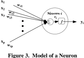
The mathematical model of a neuron used in the FFNN is depicted in Figure 3. The initial bias assigned to the neural network hidden layer and output layer is zero. The calculation process is defined as follows:

1

p

i j

j ij

v w x







; yif v( )i ₍₇₎

Where, f is the activation function of the neuron.

To model the nonlinearity of the software process more precisely, sigmoid activation and Linear activation function has been used in the hidden and output layer respectively. The connection weights have been adjusted through Levenberg-Marquardt (LM) back propagation learning algorithm.

x1

x2

x3

xp

wi1

wi2

wi3

wip

f yi

Neuron i



vi

Figure 3. Model of a Neuron

3.5

Performance measures

Variable-term prediction has been used in the proposed approach, which is commonly used in the software reliability research community [6][15]. Only part of the failure data is used to train the model and the trained model is used to predict for the rest of the failure data available in the data set. For a given execution time ti , if the predicted number of

failure is Ni’, then Ni’ is compared with the actual number of

failures i.e. Ni to calculate three performance measures such

as Average relative Error (AE), RMSE and RRMS which are defined as follows:

1

1

(( ' ) / ) *100

k

i i i

i

AE abs N N N

k 







(8)

2

1

1

[ ']

k

i i

i

RMSE N N

k 







(9)

1

1 k i i

RMSE RRMS

N k 





(10)

where kis the number of observations for evaluation.

4.

EXPERIMENTS

[image:3.595.353.533.581.678.2]

[image:4.595.343.507.80.208.2]

spurious values obtained from a network which could not train properly. In the experiment, the system is trained using 70% of the failure data for each data set and the remaining 30% software failure data are used for testing.

Table 1. Data Sets Used

Data Set Used

Errors

Detected Software Type

DS1 [1] 38 Military System

DS2 [5] 136 Realtime Command and Control DS3 [1] 54 Realtime Command and Control DS4 [1] 53 Realtime Command and Control DS5 [1] 38 Realtime Command and Control DS6 [1] 36 Realtime System

DS7 [6] 46 On-line data Entry DS8 [6] 27 Class Compiler Project DS9 [14] 100 Tandem Computer Release-1 DS10 [14] 120 Tandem Computer Release-2 DS11 [14] 61 Tandem Computer Release-3 DS12 [14] 42 Tandem Computer Release-4 DS13 [16] 234 Not Known

DS14 [6] 266 Realtime Control Application DS15 [6] 198 Monitoring and Realtime Control DS16[21] 461 Electronic switching System DS17[21] 203 Wireless network product DS18[21] 167 Bug tracking system

4.1

Effect of different encoding parameter

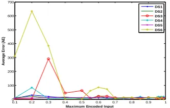
AE for all the datasets has been calculated considering raw input, exponentially encoded input and logarithmically encoded input. For the encoding functions, different values of

max

*

t _{(0.1 to 0.99) are considered. The value of} tmax _{is taken}

as the maximum possible software testing time for a data set. The effect of t*max _{value on AE is depicted in Figure 4-6 for}

[image:4.595.52.283.135.378.2]

exponential encoding function for eighteen datasets. From Figure 4-6, it is shown that for t*max _{(0.85 to 0.96), AE is less}

and consistent for all the data sets. Similarly the effect of

max

*

t _{value on AE is depicted in Figure 7-9 for logarithmic}

encoding function for eighteen datasets.

0.1 0.2 0.3 0.4 0.5 0.6 0.7 0.8 0.9 1

0 100 200 300 400 500 600

Maximum Encoded Input

A

v

e

ra

ge

E

rr

or

(A

E

)

[image:4.595.342.509.245.362.2]

DS1 DS2 DS3 DS4 DS5 DS6

Figure 4. Comparison of AE for diff value of t*

max (NEE)

0.1 0.2 0.3 0.4 0.5 0.6 0.7 0.8 0.9 1

0 50 100 150 200 250

Maximum Encoded Input

A

v

e

ra

ge

E

rr

or

(A

E

)

DS7 DS8 DS9 DS10 DS11 DS12

Figure 5. Comparison of AE for diff value of t*

max (NEE)

0.1 0.2 0.3 0.4 0.5 0.6 0.7 0.8 0.9 1

0 10 20 30 40 50

Maximum Encoded Input

A

v

e

r

a

ge

E

r

r

or

(A

E

)

DS13 DS14 DS15 DS16 DS17 DS18

Figure 6. Comparison of AE for diff value of t*

max (NEE)

From Figure 7-9, it is shown that for t*max _{(0.85 to 0.99), AE}

is less and consistent for all the data sets. It shows that prediction is less sensitive to the value of encoding parameter in this region when the upper limit on the encoded input lies somewhere in between 0.85 to 0.96 for both encoding functions. Therefore, value of upper limit on the encoded input is proposed to be 0.90.

0.1 0.2 0.3 0.4 0.5 0.6 0.7 0.8 0.9 1

0 100 200 300 400 500 600 700

Maximum Encoded Input

A

ve

ra

ge

E

rr

or

(A

E

)

[image:4.595.343.510.473.579.2]

DS1 DS2 DS3 DS4 DS5 DS6

Figure 7. Comparison of AE for diff value of t*max (NLE)

0.1 0.2 0.3 0.4 0.5 0.6 0.7 0.8 0.9 1

0 20 40 60 80 100 120 140 160 180 200

Maximum Encoded Value

A

v

e

ra

ge

E

rr

or

(A

E

)

DS7 DS8 DS9 DS10 DS11 DS12

[image:4.595.63.241.530.675.2] [image:4.595.349.502.611.737.2]

0.1 0.2 0.3 0.4 0.5 0.6 0.7 0.8 0.9 1 0

10 20 30 40 50 60 70 80

Maximum Encoded Value

A

v

e

ra

ge

E

rr

or

(A

E

)

[image:5.595.86.245.79.203.2]

DS13 DS14 DS15 DS16 DS17 DS18

Figure 9. Comparison of AE for diff value of t*max (NLE)

4.2

Effect of different encoding function

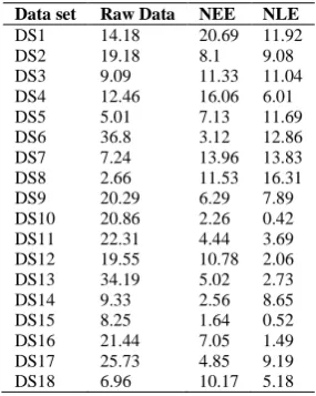
[image:5.595.329.503.80.205.2]

In this section performance of encoding functions is compared considering AE criterion for without encoding (Raw Data), Exponential encoding and logarithmic encoding and shown in Table 2. For both encoding functions the upper limit on encoded value is taken as 0.9. From the table, it can be observed that encoding improves prediction accuracy for the selected network architecture for most of data sets. Further, logarithmic encoding function found to be providing better results compared to exponential encoding function in terms of AE for many datasets. So, for further studies, logarithmic encoding has been taken as the encoding function for the actual values to scale between [0, 1].

Table 2. AE Values for different schemes

Data set Raw Data NEE NLE

DS1 14.18 20.69 11.92 DS2 19.18 8.1 9.08 DS3 9.09 11.33 11.04 DS4 12.46 16.06 6.01 DS5 5.01 7.13 11.69 DS6 36.8 3.12 12.86 DS7 7.24 13.96 13.83 DS8 2.66 11.53 16.31 DS9 20.29 6.29 7.89 DS10 20.86 2.26 0.42 DS11 22.31 4.44 3.69 DS12 19.55 10.78 2.06 DS13 34.19 5.02 2.73 DS14 9.33 2.56 8.65 DS15 8.25 1.64 0.52 DS16 21.44 7.05 1.49 DS17 25.73 4.85 9.19 DS18 6.96 10.17 5.18

4.3

Effect of number of hidden nodes

Based on the analysis in Section 4.1 and Section 4.2, logarithmic encoding function is considered for investigating the performance of the proposed approach by varying number of hidden nodes in the neural network architecture. Here, the maximum value of the encoded input is taken as 0.90. The number of neural networks considered for the investigation is considered as 10. The error plot of eighteen data sets is depicted in Figure 10. From the picture, it is clear that AE is less for most of the data sets studied if the number of hidden nodes considered as three.

2 3 4 5 6 7 8 9

0 10 20 30 40 50 60 70

Number of hidden nodes

A

v

e

ra

ge

e

rr

or

(

A

E

)

DS1 DS2 DS3 DS4 DS5 DS6 DS7 DS8 DS9 DS10 DS11 DS12 DS13 DS14 DS15 DS16 DS17 DS18

Figure 10. Effect of number of nodes on AE

4.4

Performance comparison

Based on analysis in Section 4.1- 4.3, the architecture of the system used for performance comparison consists of logarithmic encoding scheme with median combination rule. The number of hidden nodes used in the architecture is three. The number of neural networks used in the system is increased from ten to thirty. The maximum value of the encoded input value is taken as 0.85 and 0.90. Considering the above things, the proposed NLE method has been compared with [21]. The last three data sets (DS16, DS17, DS18) shown in Table 1 are considered for comparison.

4.4.1

DS16

[image:5.595.95.238.391.570.2]

The proposed model as discussed above has been applied on DS16 using 37% (i.e., the faults observed in (0, 30)), 52 %( i.e., the faults observed in (0, 30)), and 100% (i.e., the faults observed in (0, 81)) data of the dataset. The predictive ability of the proposed model in terms of RMSE and RRMS is shown in Table 3.

Table 3. Comparison of DS16

Model RMSE RRMS

G-O model (37% of data) 116.55 0.37 ISS model (37% of data) 28.16 0.09 Yamada DSS model (37% of data) 61.17 0.19 Generalized Goel NHPP model (37% of data) 113.15 0.36

Proposed NLE (37% of data)(t*max=0.90) 148.94 0.48

Proposed NLE (37% of data)(t*max=0.85) 78.01 0.25

G-O model (52% of data) 32.95 0.10 G-O model with a single CP (52% of data) 27.20 0.08 ISS model (52% of data) 20.10 0.06 ISS model with a single CP (52% of data) 19.63 0.06 Yamada DSS model (52% of data) 39.36 0.12 Generalized Goel NHPP model (52% of data) 15.69 0.05

Proposed NLE (52% of data)(t*max=0.90) 13.75 0.04

Proposed NLE (52% of data)(t*max=0.85) 23.98 0.07

G-O model (100% of data) 9.99 0.03 G-O model with two CP (100% of data) 9.35 0.03 ISS model (100% of data) 9.29 0.03 ISS model with two CP (100% of data) 9.19 0.03 Yamada DSS model (100% of data) 20.4 0.06 Generalized Goel NHPP model (100% of data) 9.16 0.03

Proposed NLE (100% of data)(t*max=0.90) 8.66 0.02

Proposed NLE (100% of data)(t*max=0.85) 6.40 0.02

[image:5.595.309.549.452.671.2]

reliability prediction, the performance of the model heavily depends upon the amount of failure data used for training. So taking 37% of data, the proposed model has worst performance due to less failure data available for training. Taking 52% and 100% of data for training, the proposed model has good performance than [21] in terms of RMSE and RRMS. Overall, when the maximum encoded value is taken as 0.85, it has better performance than 0.90. Prediction capability of the proposed NLE model is shown in Figure 11.

0 10 20 30 40 50 60 70 80 90

0 50 100 150 200 250 300 350 400 450 500

Week

C

um

m

ul

a

ti

v

e

nu

m

be

r

of

f

a

il

ure

s

[image:6.595.334.517.80.222.2]

Actual Predicted-37% Predicted-52% Predicted-100%

Figure 11. Predictive capability of DS16

4.4.2

DS17

[image:6.595.73.257.180.319.2]

The proposed model as discussed in Section 4.4 has been applied on DS17 using 66% (i.e., the faults observed in (0, 35)) and 100% (i.e., all faults observed in (0, 51)) data of the dataset. The predictive ability of the proposed model in terms of RMSE and RRMS is shown in Table 4.

Table 4. Comparison of DS17

Model RMSE RRMS

G-O model (66% of data) 29.53 0.22 ISS model (66% of data) 7.62 0.05 Yamada DSS model (66% of data) 5.62 0.04 Generalized Goel NHPP model (66% of data) 14.28 0.11

Proposed NLE (66% of data)(t*max=0.90) 10.03 0.07

Proposed NLE (66% of data)(t*max=0.85) 2.53 0.01

G-O model (100% of data) 8.74 0.06 G-O model with a single CP (100% of data) 6.79 0.05 ISS model (100% of data) 2.58 0.02 ISS model with a single CP (100% of data) 2.53 0.02 Yamada DSS model (100% of data) 3.96 0.03 Generalized Goel NHPP model (100% of data) 3.32 0.02

Proposed NLE (100% of data)(t*max=0.90) 7.49 0.05

Proposed NLE (100% of data)(t*max=0.85) 2.73 0.02

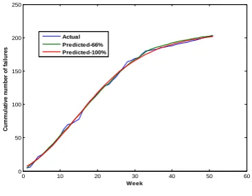
Rows from 2-5, 8-13 in Table 4 are directly taken from Table V in [21]. Predictive ability of the proposed model using 66% and 100% are shown in rows 6 and 14 in Table 4 when the maximum encoded input is taken as 0.90. Predictive ability of the proposed model using 66% and 100% are shown in rows 7 and 15 in Table 4 when the maximum encoded input is taken as 0.85. The performance of the proposed approach is found to be good when the value of maximum encoded input is taken as 0.85. Prediction capability of the proposed NLE model is shown in Figure 12.

0 10 20 30 40 50 60

0 50 100 150 200 250

Week

C

um

m

ul

a

ti

v

e

nu

m

be

r

of

f

a

il

ure

s

Actual Predicted-66% Predicted-100%

Figure 12. Predictive capability of DS17

4.4.3

DS18

The proposed model (NLE) has been applied on DS18 using 43%, 86% and 100% data of the dataset. The predictive ability of the proposed model in terms of RMSE and RRMS is shown in Table 5.

Table 5. Comparison of DS18

Model RMSE RRMS

G-O model (43% of data) 20.76 0.22 ISS model (43% of data) 20.83 0.22 Yamada DSS model (43% of data) 41.33 0.45 Generalized Goel NHPP model (43% of data) 20.59 0.22

Proposed NLE (43% of data)(t*max=0.90) 33.02 0.36

Proposed NLE (43% of data)(t*max=0.85) 27.27 0.29

G-O model (86% of data) 5.13 0.05 G-O model with a single CP (86% of data) 4.87 0.53 ISS model (86% of data) 6.92 0.07 ISS model with a single CP (86% of data) 5.73 0.06 Yamada DSS model (86% of data) 10.13 0.11 Generalized Goel NHPP model (86% of data) 5.61 0.06

Proposed NLE (86% of data)(t*max=0.90) 5.96 0.06

Proposed NLE (86% of data)(t*max=0.85) 5.98 0.06

G-O model (100% of data) 4.32 0.04 G-O model with two CP (100% of data) 4.13 0.04 ISS model (100% of data) 4.32 0.04 ISS model with two CP (100% of data) 4.10 0.04 Yamada DSS model (100% of data) 7.91 0.08 Generalized Goel NHPP model (100% of data) 4.28 0.04

Proposed NLE (100% of data)(t*max=0.90) 1.59 0.01

Proposed NLE (100% of data)(t*max=0.85) 2.00 0.02

0 5 10 15 20 25

0 50 100 150 200 250

Week

C

um

m

ul

at

iv

e

nu

m

be

r

of

f

ai

lure

s

Actual Predicted-43% Predicted-86% Predicted-100%

Figure 13. Predictive capability of DS18

[image:6.595.311.546.315.683.2] [image:6.595.49.286.441.587.2]

in terms of RMSE and RRMS. Taking 86% of training data, the proposed model has better performance than ISS model and Yamada DSS model. However RMSE and RRMS value are not significantly different from other models used in the Table 5. When 100% data used for training, the proposed model has better performance than all other models used in Table 5 in terms of RMSE and RRMS. Prediction capability of the proposed NLE model is shown in Figure 13.

According to [7], RRMS value 0.25 is an acceptable prediction value for any software reliability models. So, the proposed approach gives the acceptable value of RRMS for many cases for the three datasets used for comparison.

5.

CONCLUSION

Software reliability models are the effective techniques to estimate the duration of software testing time and release time of the software. The quality of the software is measured using these models. Neural network models are non-parametric models and proven to be the effective technique for software reliability prediction. The neural network has the ability to capture the nonlinear patterns of the failure process by learning from the failure data. The failure data are used to learn the network to develop its own internal model of the failure process using back-propagation learning algorithm. In this paper, a Feed Forward neural network with two encoding scheme such as exponential and logarithmic function has been proposed. The effect of encoding and the effect of different encoding parameter on the prediction accuracy have been investigated. The effect of number of hidden nodes on prediction accuracy has also been shown. The experimental results show that the proposed approach gives acceptable results for different data sets using the same neural network architecture.

6.

REFERENCES

[1] www.thedacs.com The Data and Analysis Centre for Software DACS.

[2] M. R. Lyu, Handbook of software reliability engineering, New York: McGraw-Hill, 1996.

[3] L.K. Hansen, P. Salamon, Neural network ensembles, IEEE Transaction on pattern Analysis and Machine Intelligence, vol. 12, no. 10, pp. 993-1001, 1990. [4] N. Karunanithi , Y.K. Malaiya , D. Whitley, Prediction

of software reliability using neural networks, Proceedings of the Second IEEE International Symposium on Software Reliability Engineering, pp. 124–130, 1991.

[5] N. Karunanithi, D. Whitley, Y.K. Malaiya, Prediction of software reliability using connectionist models, IEEE Trans Software Engg., vol. 18, no. 7, pp. 563-573, 1992. [6] N. Karunanithi, D. Whitley, Y.K. Malaiya, Using neural

networks in reliability prediction, IEEE Software, vol. 9, no. 4, pp.53–59, 1992.

[7] S.D. Conte, H.E. Dunsmore, V.Y. Shen, Software Engineering Metrics and Models, Redwood City: Benjamin-Cummings publishing Co., Inc., 1986.

[8] R. Sitte, Comparision of software–reliability-growth predictions:neural networks vs parametric recalibration,

IEEE Transactions on Reliability, vol. 48, no. 3, pp. 285-291, 1999.

[9] K.Y. Cai , L. Cai , W.D. Wang , Z.Y. Yu , D. Zhang , On the neural network approach in software reliability modeling, The Journal of Systems and Software, vol. 58, no. 1, pp. 47-62, 2001.

[10] P.M. Granotto, P.F. Verdes, H.A. Caccatto, Neural network ensembles: Evaluation of aggregation algorithms, Artificial Intelligence, vol. 163, no.2, pp. 139-162, 2005.

[11] L. Tian, A. Noore, On-line prediction of software reliability using an evolutionary connectionist model, The Journal of Systems and Software, vol. 77, no. 2, pp. 173–180, 2005.

[12] L. Tian, A. Noore, Evolutionary neural network modeling for software cumulative failure time prediction, Reliability Engineering and System Safety, vol. 87, no. 1, pp. 45–51, 2005.

[13] Q.P. Hu, Y.S. Dai, M. Xie, S.H. Ng, Early software reliability prediction with extended ANN model, Proceedings of the 30th Annual International Computer Software and Applications Conference, pp. 234-239, 2006.

[14] S.P.K. Viswanath, Software Reliability Prediction using Neural Networks, PhD. Thesis, Indian Institute of Technology Kharagpur, 2006.

[15] Y.S. Su, C.Y. Huang, Neural-Networks based approaches for software reliability estimation using dynamic weighted combinational models, The Journal of Systems and Software, vol. 80, no. 4, pp. 606-615, 2007.

[16] B. Yang, L. Xiang, A study on Software Reliability Prediction Based on Support Vector Machine, International conference on Industrial Engineering & Engineering Management, pp. 1176-1180, 2007. [17] S.H. Aljahdali, K.A. Buragga, Employing four ANNs

paradigm for Software Reliability Prediction: an Analytical study, ICGST International Journal on Artificial Inteligence and Machine Learning, vol. 8, no. 2, pp. 1-8, 2008.

[18] J. Zheng, Predicting Software reliability with neural network ensembles, Expert systems with applications, vol. 36, no. 2, pp. 2116-2122, 2009.

[19] Y. Singh, P. Kumar, Application of feed-forward networks for software reliability prediction, ACM SIGSOFT Software Engineering Notes, vol. 35, no. 5, pp. 1-6, 2010.

[20] Y. Singh, P. Kumar, Prediction of Software Reliability Using feed Forward Neural Networks, International conference on Computational Intelligence and software Engineering, pp. 1-5, 2010.