Financialisation and Crisis in an Agent Based Macroeconomomic Model

Munich Personal RePEc Archive

Financialisation and Crisis in an Agent

Based Macroeconomomic Model

Riccetti, Luca and Russo, Alberto and Gallegati, Mauro

Sapienza Università di Roma, Università Politecnica delle Marche,

Università Politecnica delle Marche

October 2013

Online at

https://mpra.ub.uni-muenchen.de/51074/

Financialisation and Crisis in an Agent Based

Macroeconomomic Model

Luca Riccetti

_{, Alberto Russo}

_{, and Mauro Gallegati}

1

_{La Sapienza Universit`a di Roma, Italy}

2

_{Universit`a Politecnica delle Marche, Ancona, Italy}

Abstract

In the present paper we analyse the role of dividends distributed by firms and banks, highlighting the effects of their increase on financial instability and macroeconomic dy-namics. During the last decades, the financialisation of nonfinancial corporations has been characterised by a shift from a “retain and reinvest” strategy to a “downsize and distribute” strategy. We will investigate such a phenomenon by varying some of the model parameters, so simulating firms’ and banks’ behaviours under alternative set-tings. On the one hand, more distributed dividends increases agents’ wealth and thus consumption may rise due to a wealth-effect. On the other hand, increasing dividends reduce firms’ net worth that may result in a strong dependence of firms’ production on bank credit; at the same time, if also banks distribute more dividends, then banks’ capital decreases and this may result in credit rationing. As we will see, financialisation through increasing dividends impacts financial (in)stability and income distribution, with relevant consequences on macroeconomic dynamics.

Keywords: agent-based macroeconomics, business cycle, leverage, payout policy, financialisation, crisis.

JEL classification codes: E32, C63, G35.

∗_{Corresponding address: Universit`a Politecnica delle Marche, Department of Economics and Social}

1

Introduction

Financialisation can be defined as “the increasing role of financial motives, financial markets, financial actors and financial institutions in the operation of domestic and international eco-nomies” Epstein (2005, p.3). In this paper we focus on the role of dividends paid by firms and banks to shareholders as one of the phenomenon that increases the weight of finance in the whole economic system.

Regarding the modeling framework we analyse the effects of financialisation on macroe-conomic dynamics in an agent based macroemacroe-conomic setting, as described in Riccetti et al. (2012), in which the macroeconomy is a complex system populated by heterogeneous agents (households, firms and banks) which directly interact in different markets (goods, labour, credit, and bank deposits). There are two policy makers: the government and the central bank. In this context, aggregate regularities emerge from the “bottom up” (Epstein and Ax-tell, 1996) as statistical properties at the meso and macro levels that derive from the (simple and adaptive) individual behavioral rules and the interaction mechanisms which describe the working of markets (Tesfatsion and Judd, 2006; LeBaron and Tesfatsion, 2008).

As we will see, increasing dividends can make the system financially unstable and can have relevant consequences on income distribution. In fact, firms that only pay dividends are largely extinct.1

Repurchases are increasingly used in place of dividends, even for firms that continue to pay dividends. On these bases, Skinner (2008) suggests that repurchases are now the dominant form of payout. To be more precise, aggregate real dividends paid by industrial firms increased over the past two decades even though, as shown by Fama and French (2001), the number of dividend payers decreased by over 50%; in particular, DeAngelo et al. (2004) find that (i) the reduction in payers occurs almost entirely among firms that paid very small dividends, and (ii) increased real dividends from the top payers swamp the modest dividend reduction from the loss of many small payers. Such a behaviour reflects high and increasing concentration in the supply of dividends which, in turn, reflects high and increasing concentration of earnings. For instance, the 25 firms that paid the largest dividends in 2000 account for a majority of the aggregate dividends and earnings of industrial firms. (DeAngelo et al., 2004).

Moreover, “over the decade 2001-2010, the 500 corporations in the S&P 500 Index (rep-resenting about 75 percent of US stock-market capitalization) expended not only 40 percent of their profits on cash dividends – the normal mode of rewarding shareholders – but also another 54 percent on stock buybacks, the purpose of which is to give a manipulative boost to a company’s own stock price” (Lazonick, 2013). Morevover, large scale payments of di-vidends has continued during the “financial crisis”, in spite of widely anticipated credit losses (Acharya et al, 2011). According to Admati (2012), “money paid to shareholders (or

man-1

agers) is no longer available to pay creditors. Share buybacks and dividend payments reduce the banks’ ability to absorb losses without becoming distressed. When a large “systemic” bank is distressed, the ripple effects are felt throughout the economy”. Therefore, the lar-ger the dividends distributed to shareholders the higher the systemic risk due to financial contagion.

As for the relationship between financialisation and distribution, it may be expected that shareholders’ demand for higher distributed profits may be passed through to workers resulting in a decline of the wage share, as stressed by Boyer (2000). According to Hein (2011, p. 298), “in the medium to the long run increasing shareholder power favours redistribution at the expense of the labour income share”. While numerous studies have detected the declining behaviour of the labour share in many countries, only a few contributions investigated the relationship between financialisation and distribution. For instance, D¨unhaupt (2013) seeks to explore the relationship between financialisation and labour’s share of income using a time-series cross-section data set of 13 countries over the time period from 1986 until 2007. The results suggest that there is indeed a relationship between increasing dividend and interest payments of non-financial corporations and the decline of the share of wages in national income.2

The increase of financial instability as well as the decline of the wage share are the con-sequence of relevant changes in the macroeconomic system of advanced countries during the

neoliberal era (Russo, 2012). After the stagflation of the 1970s, a series of political decisions have changed the institutional and organisational settings of capitalist accumulation emerged after the WWII: the institutional arrangement of capitalist accumulation emerged after the 1970s has resulted in a partial return to the pre-Great Depression “free-market” capitalism, removing the constraints to financial and economic activity implemented by governments in response to the post-1929. After the early XX century belle ´epoque, a new one emerged dur-ing the last decades of the same century with some resembldur-ing features as the expansion of finance, growing inequality and increasing instability. There are, then, some relevant simil-arities between the recent crisis and the post-1929 one, even though differences are perhaps more numerous, especially if we consider the pervasiveness of finance in the economic and social life. Our contribution focuses on the increasing role of finance in the economy, through investigating firms’ and banks’ dividend policies.

Analysing the US macroeconomic trends since the 1960s, van Treeck (2009, p.13) shows some of the main changes occurred after the 1970s. We summarise these findings - relative to the two sub-periods, until the early 1980s and since the early 1980s - as follows:

• the income inequality was relatively low and roughly stable, then it has drastically increased (to levels comparable to the 1920s);

2

• the personal net worth-to-income ratio was relatively stable or slightly decreasing, then it has strongly increased;

• the personal saving rate was relatively high and slightly increasing, then it has drastically declined (reaching negative values for the first time since the early 1930s);

• the personal debt-to-income ratio was relatively low and roughly stable, then it has drastically increased;

• non-financial corporations retained a large and roughly stable fraction of their net profits, then they have heavily increased the dividend-payout ratio;

• the growth rate of net capital stock displayed cyclical movements around a relatively high trend, then it has shown an overall declining trend (with the relevant exception of the “new economy” boom of the 1990s);

• the contribution of the net new equity issues to the financing of fixed capital investment by non-financial corporations was small but positive, then it turned to be negative and very large in absolute value;

• firms’ debt-to-capital ratio was relatively low, then it has increased.

Therefore, the post-1970s deregulation wave has increased inequality and indebtedness (both for households and firms), promoting a broader role for finance in the working of the economy. For instance, the US financial corporations’ pre-tax profit rose from an average of 13.9% of all corporate profits in the 1960s to 25.3% in the 1990s and 36.8% in the period 2000-2006; in general, from the 1970s to the 1990s, there was an increase of the share of national income received by financial institutions and financial wealth’s holders in the majority of OECD countries (Epstein and Jayadev, 2005).

real capital accumulation; second, increased financial payments leave firms with fewer funds to invest and shorten the planning horizon of firms’ management.

According to Lazonick and O’Sullivan (2000), the financialisation of nonfinancial corpor-ations has been characterised by a shift from a retain and reinvest strategy to a downsize and distribute strategy; that is, management strategies have changed focussing more on the maximisation of shareholder value and less on long-term growth. In fact, the profit share increase of recent decades has been accompanied by the stagnation of real investment and a sharply increase of interest payments, dividend payments and stock buybacks (also mergers and acquisitions may be considered).

Stockhammer (2004) confirms that over the past decades the financial investment of nonfin-ancial corporations has been rising and the accumulation of capital goods has been declining. According to this author, the “shareholder revolution” and the development of a market for corporate control have shifted power to shareholders and thus changed management priorities, so leading to a reduction of growth rates. From the analysis of the time series of aggregate investment for the USA, the UK, France and Germany, it results that financialisation has been responsible for a slowdown of accumulation (in particular, for the first three countries). Similar results have been reached by Crotty (2005), according to which nonfinancial cor-porations have increased financial investments as response to high interest rates and to low rates of profit associated to real investments, and Dumenil and Levy (2005), according to which the growth rate of real capital accumulation depends on that of retained profits (that is, profit after interest and dividend payments), which is diminished in recent decades.

All in all, financialisation has been a fundamental factor behind the recovery of profits from the 1980s in the leading capitalist economy as well as a phenomenon involved in a slowdown of real capital accumulation. Unsurprisingly, the average growth rate of most advanced countries, during the US financial expansion of the post-1970s, has been lower than in the post-WWII “regulated capitalism”.

The paper is organised as follows. After this Introduction, we present the modelling framework in Section 2. In Section 3 we discuss simulation results: first, we briefly de-scribe the dynamic behaviour of the model in the baseline scenario; then, we perform some computational experiments to assess the relevance of dividends on financial instability and macroeconomic dynamics. Finally, Section 4 provides some concluding remarks.

2

The model

This paper is based on the model reported in Riccetti et al. (2012). Our economy evolves over a time span t = 1,2, ..., T and is composed by households (h = 1,2, ..., H), firms (f = 1,2, ..., F), banks (b = 1,2, ..., B), a central bank, and the government. Agents are boundedly rational and live in an incomplete and asymmetric information context, thus they follow simple rules of behaviour and use adaptive expectations.

Agents interact in four markets: (i) credit market; (ii) labour market; (iii) goods market; (iv) deposit market. The interaction between the demand (firms in the credit and labour markets, households in the goods market, and banks in the deposit market) and the supply (banks in the credit market, households in the labour and deposit markets, and firms in the goods market) sides of the four markets follows a common decentralized matching protocol, even if each agent in the demand side observes a list of potential counterparts in the supply side and chooses the most suitable partner according to some market-specific criteria. In particular, the interaction develops in the following way: a random list of agents in the demand side is set, then the first agent in the list observes a random subset of potential partners, whose size depends on a parameter 0< χ≤1 (which proxies the degree of imperfect information), and chooses the cheapest one. After that, the second agent on the list performs the same activity on a new random subset of the updated potential partner list. The process iterates till the end of the demand side list. Subsequently, a new random list of agents in the demand side is set and the whole matching mechanism goes on until either one side of the market (demand or supply) is empty or no further matchings are feasible because the highestbid (for example, the money till available to the richest firm) is lower than the lowest ask (for example, the lowest wage asked by till unemployed workers).

Now, we briefly explain the main features of the four markets. However, for a detailed description of the markets, we refer to Riccetti et al. (2012).

2.1

Markets

2.1.1 Credit market

Bf td =Af t·lf t (1)

The evolution of the leverage target changes according to expected profits and inventories: if expected profits are above expected interest rate and there are few inventories, the firm enlarges its target leverage, and viceversa. Therefore, we implement a version of the Dynamic Trade-Off Theory (Flannery and Rangan, 2006) based onadaptive rules of firm’s behaviour.3

Banks set their credit supplyBd

bt depending on their net worth Abt, deposits Dbt, and the

quantity of money provided by the central bank mbt. However, they must comply with some

regulatory constraints: the maximum admissible leverage, the maximum percentage of capital to be invested in lending activities and the maximum risk concentration (that is, banks lend to a single firm up to a maximum fractionβ of the total amount of the credit Bd

bt).

Under asymmetric information (Stiglitz and Weiss, 1981), bankb charges an interest rate on the firm f at time t according to the following equation:

ibf t =iCBt+ ˆibt+ ¯if t (2)

where iCBt is the nominal interest rate set by the central bank at time t, ˆibt is a

bank-specific component, and ¯if t = ρlf t/100 is a firm-specific component, that is a risk premium

on firm target leverage (with ρ >0).

The bank-specific component decreases if the bank did not manage to lend to firms all the credit supply. Indeed, at the end of the interaction mechanism, each firm ends up with a creditBf t ≤Bf td and each bank lends to firms an amount Bbt ≤Bbtd. The difference between

desired and effective credit is equal to Bd

f t−Bf t = ˆBf t and Bbtd −Bbt = ˆBbt, for firms and

banks respectively.

Moreover, we assume that banks try to invest residual credit supply in government securities. If the sum of desired government bonds exceeds the amount of outstanding public debt then the effective investment is proportionally rescaled. Instead, if public debt exceeds the banks’ desired demand, then the central bank buys the residual amount.

2.1.2 Labour market

Government, firms and households interact in the labour market. On the demand side, first of all, the government hires a fraction g of households. The remaining part is available for working in the firms. Firm’s f labour demand depends on available funds, that is net worth and bank credit: Af t+Bf t.

On the supply side each worker posts a wage wht which increases if he/she was employed in

the previous period and viceversa. Moreover, the required wage has a minimum related to

3

the price of a good.

As a result of the decentralized matching between labour supply and demand, each firm ends up with a number of workersnf t and a residual cash (insufficient to hire an additional worker)

and a fraction of households may remain unemployed. The wage of unemployed people is set equal to zero.

2.1.3 Goods market

Subsequently, households and firms interact in the goods market. On the demand side, households set the desired consumption on the basis of their disposable income and wealth. Firms produce consumption goods on the basis of hired workers as follows:

yf t=φ·nf t (3)

whereφ≥ 1 is a productivity parameter. They put in the goods market their current period production and previous period inventories ˆyf t−1. The selling price increases if in the previous period the firm managed to sell all the output, while it reduces if it had positive inventories. Moreover, the minimum price at which the firm want to sell its output is set such that it is at least equal to the average cost of production, that is ex-ante profits are at worst equal to zero.

As a consequence of the interaction between the supply and demand sides in the goods market, each household ends up with a residual cash, that is not enough to buy an additional good and that she will try to deposit in a bank. At the same time, firms may remain with unsold goods (inventories), that they will try to sell in the next period.

2.1.4 Deposit market

Banks and households interact in the deposit market. Banks represent the demand side and households are on the supply side. Banks offer an interest rate on deposits according to their funds requirement: if a bank exhausts the credit supply by lending to private firms or government then it decides to increase the interest rate paid on deposits, so to attract new depositors, and viceversa. However, the interest rate on deposits can increase till a maximum given by the policy raterCBt which is both the rate at which banks could refinance from the

central bank and the rate paid by the government on public bonds.

offers an adequate interest rate. A household that decides to not deposit her money in a bank signals a preference for liquidity.

2.2

Profits, dividends and wealth dynamics

2.2.1 Firms

At the end of the interaction in the credit, labour and goods markets, every firmf calculates its profit/loss:

πf t=pf t·y¯f t−Wf t−If t (4)

where pf t is the price set by the firm f on its goods, ¯yf t are the sold goods, Wf t is the

sum of wages paid to employed workers, andIf t is the sum of interests paid on bank loans.

Firms pay a proportional tax τ on positive profits; however, firms can subtract previous negative profits in the calculation of the tax base. After taxes, we indicate net profits with ¯

πf t.

Finally, firms pay a percentage ˆδf t as dividends on positive net profits. The fraction 0≤δˆf t ≤

1 evolves according to the following rule:

ˆ

δf t = ¯δf +δf t (5)

with:

δf t = 8

<

:

δf t−1·(1−α·U(0,1)), if ˆyf t= 0 and yf t>0

δf t−1·(1 +α·U(0,1)), if ˆyf t>0 or yf t= 0

(6)

and with 0< α < 1 as adjustment parameter. The previous equation means that dividends go down if in the previous period the firm produces and sells all the goods (no inventories), then it wants to retain a larger share of profits to enlarge the production, and viceversa. The profit net of taxes and dividends is indicated by ˆπf t. In case of negative profits ˆπf t =πf t.

Thus, the evolution of firmf’s net worth is given by:

Af t = (1−τ′)·[Af t−1+ ˆπ_{f t}] (7)

where τ′ _{is the tax rate on wealth (applied only on wealth exceeding a threshold ¯τ}′_{·p¯, that}

is a multiple of the average goods price).

IfAf t≤0 then the firm goes bankrupt and a new entrant replaces the bankrupted agent

according to a one-to-one replacement. Banks linked to defaulted firms lose a fraction of their loans calculated as (Af t+Bf t)/Bf t: this is the recovery rate.

2.2.2 Banks

As a result of interaction in the credit and the deposit markets, the bank b’s profit is equal to:

πbt =intbt+i

Γ

t ·Γbt−iDbt−1·Dbt−1−it_CB·m_bt−bad_bt (8) where intbt represents the interests gained by bank b on lending to non-defaulted firms, i

Γ

t

is the interest rate on government securities Γbt, iDbt−1 is the interest rate paid on the sum of deposits Dbt−1, itCB is the interest rate paid on the amount of money mbt required to the

Central Bank, and badbt is the amount of “bad debt” due to bankrupted firms. Bad debt

is the loss given default of the total loan, that is a fraction 1 less the recovery rate (see the previous subsection) of the loan.

Banks pay a proportional tax τ on positive profits; however, they subtract previous negative profits in the calculation of the tax base. We indicate net profits with ¯πbt.

Finally, banks pay a percentage ˆδbt as dividends on positive net profits. The fraction 0 ≤

ˆ

δbt ≤1 evolves according to the following rule:

ˆ

δbt = ¯δb +δbt (9)

where:

δbt = 8

<

:

δbt−1 ·(1−α·U(0,1)), if B_bt>0 and ˆB_bt = 0

δbt−1 ·(1 +α·U(0,1)), if B_bt= 0 or ˆB_bt >0

(10)

That is, if the bank does not manage to lend the desired supply of credit then it decides to distribute more dividends (because it does not need high reinvested profits), and viceversa. The profit net of taxes and dividends is indicated by ˆπbt. In case of negative profits

ˆ

πbt =πbt.

Thus, the bankb’s net worth evolves as follows:

Abt = (1−τ′)·[Abt−1+ ˆπbt] (11)

where τ′ _{is the tax rate on wealth (applied only on wealth exceeding a threshold ¯τ}′ _·p¯,

that is a multiple of the average goods price).

IfAbt ≤0 then the bank is in default and a new entrant takes its place. Households linked

to defaulted banks lose a fraction of their deposits (the loss given default rate is calculated as 1−(Abt+Dbt)/Dbt). The initial net worth of the new entrant is a multiple of the average

goods price. Moreover, the initial bank-specific component of the interest rate (ˆibt) is equal

to the mean value across banks.

2.2.3 Households

Aht = (1−τ′)·[Aht−1 + (1−τ)·w_ht+div_ht+intD_ht−c_ht] (12)

where τ′ _{is the tax rate on wealth (applied only on wealth exceeding a threshold ¯τ}′ _·p¯,

that is a multiple of the average goods price), τ is the tax rate on income, wht is the wage

gained by employed workers, divht is the fraction (proportional to the household h’s wealth

compared to overall households’ wealth) of dividends distributed by firms and banks net of the amount of resources needed to finance new entrants (hence, this value may be negative),

intD

ht represents interests on deposits, and cht is the effective consumption. Households linked

to defaulted banks lose a fraction of their deposits as already explained.

2.3

Government and central bank

Government’s current expenditure is given by the sum of wages paid to public workers (Gt)

and the interests paid on public debt to banks. Moreover, government collects taxes on incomes and wealth and receives interests gained by the central bank. The difference between expenditures and revenues is the public deficit Ψt. Consequently, public debt is Γt = Γt−1+Ψt.

Central bank decides the policy rate iCBt and the quantity of money to put into the

system in accordance with the interest rate. In order to do that, the central bank observes the aggregate excess supply or demand in the credit market and sets an amount of moneyMt

to reduce the gap in the subsequent period of time.

3

Simulations

We explore the dynamics of the model by means of computer simulations. We refer to Riccetti et al. (2012) for the details about the parameter setting, the initial conditions and the results of the baseline model that we will sum up in the next subsection.

3.1

Baseline model results

demand, while on the other hand reduces firms’ profits, possibly causing the inversion of the business cycle. Then, we can notice a “real” economy engine given by the dynamic relation between the unemployment and the profit rate, enlarged by a financial accelerator mechan-ism. The “real” mechanism is that an increase of profits boosts the expansion of the economy and then a fall of the unemployment rate follows; the low unemployment increases wages, so firms try to save on production costs reducing labour demand. This results in a rise of unemployment that lowers the profit rate at the subsequent period due to a lack of aggregate demand. However, the presence of unemployed people decreases wages and this makes firms to hire a larger number of workers, so boosting the beginning of a new expansionary phase of the business cycle.

Firms’ leverage and banks’ exposure are the financial drivers that enlarge business fluctu-ations: growing firms ask for more credit and, if banks extended new loans, then they expand the production; subsequently, the low unemployment fosters wages that, together with the rise of interest payments on an increasing debt, reduces firms’ profitability. Thus, the busi-ness cycle reverses and financial factors amplify the recession, indeed the relatively low level of profits with respect to interest payments induces a deleveraging process. According to the empirical evidence (for example, Kalemli-Ozcan et al., 2011), there is a negative but mod-est correlation between firms’ leverage and the unemployment rate, while there is a more significant negative correlation between banks’ exposure and unemployment. Then, banks’ capitalization is the most important determinant of credit conditions, so influencing firms’ leverage and the macroeconomic evolution.

The business fluctuations are mitigated by the government, representing an acyclical sec-tor, that plays a central role to reduce the output volatility through stabilizing the aggregate demand. However, in 5 out of 1000 “short” simulations and in 2 out of 100 “long” ones, the system is characterized by large and extended crises, that is the average unemployment rate reaches values above the 20%. Differently from the usual business cycle mechanism, the re-duced wages due to growing unemployment does not reverse the cycle, but generates a lack of aggregate demand that amplifies the recession in a vicious circle for which the fall of purchas-ing power prevents firms to sell commodities, then firms decrease production, unemployment continues to rise, and the recession further deteriorates.

3.2

Dividend analysis

In this section we investigate the effects of modifying the percentage of dividends paid on net profits: in particular, we change the parameters ¯δf (see equation 5) and ¯δb (equation 9). In

the baseline model ¯δf = ¯δb = 0. When we modify both parameters at the same level, for

simplicity we will call them ¯δ, that is ¯δ= ¯δf = ¯δb.

T=150, for an overall amount of 1000 simulations.

The second study checks the impact of the parameter over “long” time horizon simulations. That is, we run 100 Monte Carlo simulations with T=500 for ¯δ = 0.45 and ¯δ= 0.30, in order to compare these results with the results emerging from the 100 simulations of the baseline model over the “long” time span. Moreover, we analyze the impact of different values of ¯δf

and ¯δb, and in particular we explore two combinations: (i) ¯δf = 0.45 and ¯δb = 0, (ii) ¯δf = 0

and ¯δb = 0.45. Overall, we perform an additional set of 400 simulations.

Firstly, we perform the sensitivity analysis on the parameter ¯δthat influences the percent-age of dividends paid by firms and banks. As already said, we run 1000 simulations for 10 different values of ¯δ, from 0 to 0.45 with 0.05 step. At first, we do not consider simulations with large crisis, defined as simulations in which the mean unemployment rate exceeds the 20%.

Figure 1 displays the impact of parameter ¯δ on the following variables: (i) the dividend amount on GDP, (ii)-(iii) the dividend percentage on firms and banks net profits, (iv) the unemployment rate, (v) the unemployment volatility, (vi) firms and banks default rate, (vii) firms and banks overall profits, (viii) firms and banks total assets, (ix) firms leverage (com-puted as liabilities on net worth) and banks exposure, (x) the overall credit mismatch (that is the difference between the aggregate credit supply and the aggregate credit demand), (xi) the wage share, and (xii) the inflation rate. As expected, when ¯δ grows, the dividends increase both on GDP and on profits. The dividends growth makes unemployment worse and worse. This is due to a decrease of reinvested profits, thus firms’ net worth diminishes: firms have less disposable cash, and then they are able to hire a smaller number of workers. However, this effect is quite small for 0≤δ¯≤0.35, because the increase of firms’ profits. Higher profits make firms to increase their leverage level and, for relatively small level of dividends, this partially counteracts the impact of the reduced net worth on the overall assets value. Then, the mean unemployment rate exhibits a slight increase, even if the high leverage makes the economy less stable as shown by the rise of the unemployment rate’s standard deviation. The low mean unemployment rate and the increasing “consumption” of profits (because of the high dividend yield) make firms’ profits higher and higher supporting the macroeconomic system, as already said. Obviously, the increase of the profit share is connected with a decreasing wage share; moreover, this feature reduces the inflation rate.

Instead, for`u ¯δ >0.35 firms’ assets value steepely decreases (see firms total assets panel). This is due to the joint impact of the reduced firms’ net worth and of the reduced banks’ supplu of credit. Indeed, when dividends are very high, also banks net worth decreases, reducing the credit supply (even if banks’ leverage goes up) and causing a growing credit rationing (see the credit mismatch panel), forcing firms to reduce their leverage. In this setting, the mean unemployment rate largely grows and also the volatility of the macroeconomic system goes up, increasing the number of firm and bank defaults, even if the system is still profitable.

situ-Figure 1: Sensitivity analysis on the impact of the parameter ¯δ – from 0 to 0.45 with step 0.05 – on (i) dividend amount on GDP, (ii) dividend percentage on firms net profits, (iii) dividend percentage on banks net profits, (iv) unemployment rate, (v) unemployment volatility, (vi) firms (indicated by a “o”) and banks (“x”) default rate, (vii) firms and banks profits, (viii) firms and banks assets, (ix) firms leverage and banks exposure, (x) credit mismatch, (xi) wage share, (xii) inflation rate.

0 0.1 0.2 0.3 0.4

0 0.02 0.04 0.06 0.08

dividends on GDP

0 0.1 0.2 0.3 0.4

0.2 0.4 0.6 0.8 1

firms dividends on net profits

0 0.1 0.2 0.3 0.4

0.2 0.4 0.6 0.8 1

banks dividends on net profits

0 0.1 0.2 0.3 0.4

0.08 0.1 0.12 0.14 0.16 unemployment rate

0 0.1 0.2 0.3 0.4

0.02 0.03 0.04

unemployment rate std

0 0.1 0.2 0.3 0.4

−800 −600 −400 −200 0 credit mismatch

0 0.1 0.2 0.3 0.4

0.57 0.59 0.61 0.63 0.65 wage share

0 0.1 0.2 0.3 0.4

0.016 0.018 0.02

inflation

0 0.1 0.2 0.3 0.4

0.05 0.08 0.11 0.14

firms and banks defaults

0 0.1 0.2 0.3 0.4 0

0.01 0.02 0.03

0 0.1 0.2 0.3 0.4

20 40 60 80

firms and banks profits

0 0.1 0.2 0.3 0.4 20

30 40 50

0 0.1 0.2 0.3 0.4

650 700 750 800 850

firms and banks total assets

0 0.1 0.2 0.3 0.4 400

500 600 700 800

0 0.1 0.2 0.3 0.4

1.4 1.5 1.6 1.7 1.8

firms and banks leverage

0 0.1 0.2 0.3 0.4 2

ations. Indeed, the rise of unemployment can cause a large crisis due to a lack of aggregate demand, thus implying a fall of the firms’ profit rate and triggers the recession spiral already explained in section 3.1. In Table 1, we report some statistics about all simulations, that is including the “large crisis” ones. For some values of ¯δ there are no large crises; in these cases the numbers in Table 1 are the same as in Figure 1. We can observe that the only significant changes happen when firms and banks distribute a large fraction of profits by dividends, that is for ¯δ = 0.45, when three large crises happen, and two of these are situations in which the economy remains trapped in an almost total disruption of the private sector. In the other cases, the same comments provided about Figure 1 hold: the economy is almost stable if 0 ≤ δ¯ ≤ 0.35 and significantly changes its state for ¯δ > 0.35. Indeed, if ¯δ > 0.35, overall dividends are above the 5% of GDP, firms distribute over the 70% of their net profits and banks distribute over the 60% of their net profits, the macroeconomic system becomes weaker and weaker, with very bad outcomes: the mean unemployment rate varies from about 10% (for 0≤δ¯≤0.35) to 15% (when ¯δ= 0.45), the rate of firm defaults grows from less than 8% to more than 14%, and the rate of bank defaults increases from about 1% to almost 4.5%.

Table 1: Sensitivity analysis for parameter ¯δ from 0 to 0.45: 100 simulations for each value, time span 101-150.

¯

δ _{(%) 0 5 10 15 20 25 30 35 40 45}

Sim. with large crisis 0 1 1 0 2 0 0 0 0 3 Dividends on GDP (%) 1.1 1.4 1.7 2.1 2.6 3.1 3.8 4.5 5.4 6.0 Mean unemployment rate (%) 9.8 10.8 11.1 10.7 11.3 10.6 10.9 11.3 12.9 15.1 Unemployment std. dev. (%) 2.0 2.1 2.2 2.2 2.7 2.5 2.9 3.1 3.8 3.8 Wage share (%) 63.5 63.3 63.0 62.8 62.5 62.2 61.6 60.9 59.5 58.6 Firm default rate (%) 6.5 7.5 7.6 6.3 7.3 6.0 7.3 7.9 9.0 14.2 Bank default rate (%) 0.62 1.66 1.69 0.64 1.96 0.94 1.10 1.12 1.57 4.49

To better check for the presence of large crises, we perform a battery of Monte Carlo simulations over a “long” time horizon T=500 (excluding the first 100 time steps from the data analysis, which have the role of initializing the system). In section 3.1 we commented the baseline case, that is ¯δ= 0. Now we propose four new experiments, each with 100 simulations:

• δ¯= 0.45;

• δ¯= 0.30;

• δ¯f = 0.45 and ¯δb = 0;

• δ¯f = 0 and ¯δb = 0.45.

times over 100 Monte Carlo simulations, while for ¯δ = 0.45 we count 26 simulations with large crises, that is with a mean unemployment rate above 20%. 12 times out of these 26 simulations, the economy remains trapped in a substantial disruption of the private sector, that is with an unemployment rate above 50% (consider that we assume the public sector to hire 1/3 of the households, thus the maximum unemployment is the 66.6%). Instead, in other 11 times simulations present a mean unmeployment rate slightly above 20%. In the last three cases, the macroeconomy suffers from a long period of large unemployment, but in the “long run” the system goes back to the “standard” statistical equilibrium, with a cyclical behavior around a “reasonable” rate of unemployment.

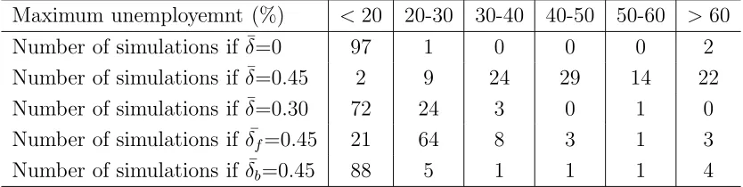
To assess the possibility of short periods of large unemployment even in simulations classi-fied as without large crisis, we check the maximum unemployment registered betweent= 101 and t = 500. Table 2 contains the number of simulations with a maximum unemployment rate included in the following ranges: less than 20%, between 20% and 30%, between 30% and 40%, between 40% and 50%, between 50% and 60%, and above 60%. According to the data presented in the table, it is almost impossible that an economy does not face some periods of strong crisis, when the dividend yield becomes too high (for instance above ¯δ= 0.45). We repeat the previous analysis in the other three settings itemized above. Indeed, the analysis on a time horizon equal toT = 150 showed that the economic system does not present very relevant problems till ¯δ = 0.35, then we decide to check if the system is stable even in the long run, for a value of ¯δ below this threshold (that is ¯δ = 0.3). For the same reason we also check for heterogeneity of behaviours between firms and banks: in the short run analysis we showed that large crises appear when firms do not have enough money to hire workers, both from internal funds and from bank credit; but, it could also happen that firms with high dividends reduce their net worth, but banks have more money to lend ( ¯δf = 0.45 and

¯

δb = 0) or, conversely, that banks with high dividends reduce their credit supply, but firms

have enough net worth ( ¯δf = 0 and ¯δb = 0.45) and a large crisis is avoided. In line with what

we found in the short run analysis, big crises largely reduce compared to the case of ¯δ= 0.45. However, we can confirm that the probability to face one or more periods of large unemploy-ment (also in a non large crisis simulation) increases when dividends grow, even if either firms or banks enlarge their dividends. Moreover, the Monte Carlo with ¯δf = 0.45, that is the worst

case excluding ¯δ = 0.45, presents some simulations in which the mean unemployment rate is slightly above 20%, differently from the “standard” case.

Table 2: Maximum unemployment for different values of ¯δ: 100 simulations for each value, time span 101-500.

Maximum unemployemnt (%) <20 20-30 30-40 40-50 50-60 >60 Number of simulations if ¯δ=0 97 1 0 0 0 2 Number of simulations if ¯δ=0.45 2 9 24 29 14 22 Number of simulations if ¯δ=0.30 72 24 3 0 1 0 Number of simulations if ¯δf=0.45 21 64 8 3 1 3

Number of simulations if ¯δb=0.45 88 5 1 1 1 4

excessive growth of the dividends enlarges financial fragility and consequently macroeconomic instability, that is the probability to face, sooner or later, a big economic crash with a high unemployment rate.

4

Concluding remarks

After the stagflation of the 1970s, a series of political decisions have changed the institu-tional and organisainstitu-tional settings of capitalist accumulation emerged after the WWII: the institutional arrangement of capitalist accumulation emerged after the 1970s has resulted in a partial return to the pre-Great Depression “free-market” capitalism, removing the constraints to financial and economic activity implemented by governments in response to the post-1929. Our contribution focuses on the increasing role of finance in the economy, through focussing on firms’ and banks’ dividend policies.

Financialisation of nonfinancial corporations has been characterised by a shift from a “re-tain and reinvest” strategy to a “downsize and distribute” strategy; that is, management strategies have changed focussing more on the maximisation of shareholder value and less on long-term growth. In fact, the profit share increase of recent decades has been accompanied by the stagnation of real investment and a sharply increase of interest payments, dividend payments and stock buybacks (also mergers and acquisitions may be considered). The “share-holder revolution” and the development of a market for corporate control have shifted power to shareholders and thus changed management priorities, so leading to a reduction of growth rates. All in all, financialisation has been a fundamental factor behind the recovery of profits from the 1980s in the leading capitalist economy as well as a phenomenon involved in a slow-down of real capital accumulation. Unsurprisingly, the average growth rate of most advanced countries, during the US financial expansion of the post-1970s, has been lower than in the post-WWII “regulated capitalism”.

finan-cialisation, which involved firms along the shift from a “retain and reinvest” approach to a “downsize and distribute” strategy, by varying some of the model parameters, so simulating firms’ and banks’ behaviours under alternative settings. As for the modelling framework, we perfomed our analysis in an agent based setting in which the macroeconomy is a complex sys-tem populated by heterogeneous agents (households, firms and banks) which directly interact in different markets (goods, labour, credit, and bank deposits). Then, there are two policy makers: the government and the central bank. In this context, aggregate regularities emerge from the “bottom up” as statistical properties at the meso and macro levels that derive from the (simple and adaptive) individual behavioural rules and the interaction mechanisms which describe the working of markets.

Model simulations show that when firms and banks decide to increase the fraction of profits to be distributed as dividends, the rate of unemployment tends to rise. Higher unemployment results in lower wages that, in turn, may have two different effects: on the one hand, it reduces workers’ consumption; on the other hand, it reduces firms’ production costs and, if a part of dividends finances consumption, then the firms’ profit rate may rise. This implies a decline of the wage share (because wages decrease at a faster rate than price inflation). So, this type of “financialisation” of the macroeconomic system may work based on the substitution of a part of wages with a fraction of dividends in the financing of consumption. This is, however, a temporary solution, given that the reduced fraction of retained profits results in a decrease of firms’ and banks’ net worth. In this scenario, firms need more credit (due to a lower level of internal funds) while banks are characterised by a reduced amount of credit supply. In this situation firms may face credit rationing and they may be forced to reduce their leverage. As a consequence, firms cannot hire the desired number of workers and the unemployment rate goes up, while the volatility of the financial and of the macroeconomic system increases. Moreover, the rise of unemployment further deteriorates the problem of aggregate demand insufficiency and this may result in an extended crisis.

References

[1] Acharya V.V., Gujral I., Kulkarni N., Shin H.S. (2011), “Dividends and Bank Capital in the Financial Crisis of 2007-2009”, NBER Working Paper No. 16896, National Bureau of Economic Research.

[2] Admati A. (2012), “Why the bank dividends are not a good idea”, Reuters blog http://blogs.reuters.com/great-debate/2012/03/14/why-the-bank-dividends-are-a-bad-idea/

[3] Boyer R. (2000), “Is a finance-led growth regime a viable alternative to Fordism? A preliminary analysis”,Economy and Society, 29:111-145.

[4] Brav A., Grahama J.R., Campbell RR.H., RMichaely R. (2008), “Payout policy in the 21st century”, Journal of Financial Economics, 77: 483-527.

[5] Crotty J. (2005), “The Neoliberal paradox: the impact of destructive product market competition and ’modern’ financial markets on nonfinancial corporation performance in the Neoliberal era”, pp. 77-101, in: Epstein G. (ed.), Financialization and the World Economy, Cheltenham and Northampton, Edward Elgar.

[6] DeAngelo H., DeAngelo L., Skinner D.J. (2004), “Are dividends disappearing? Di-vidend concentration and the consolidation of earnings”,Journal of Financial Economics, 72:425-456.

[7] Delli Gatti D., Gallegati M., Greenwald B., Russo A., Stiglitz J.E. (2010), “The financial accelerator in an evolving credit network”, Journal of Economic Dynamics and Control, 34(9): 1627-1650.

[8] Denis D.J., Osobov I. (2008), “Why do firms pay dividends? International evidence on the determinants of dividend policy”, Journal of Financial Economics, 89: 62-82.

[9] Dum´enil G., L´evy D. (2005), “Costs and benefits of Neoliberalism: A class analysis”, pp. 17- 45, in: Epstein G. (ed.), Financialization and the World Economy, Cheltenham and Northampton, Edward Elgar.

[10] D¨unhaupt P. (2013), “The effect of financialization on labor’s share of income”, Working Paper No. 17/2013, Institute for International Political Economy Berlin.

[11] Epstein G. (2005), “Introduction: Financialization and the world economy”, in Epstein G. (ed.), Financialization and the World Economy, Cheltenham and Northampton: Ed-ward Elgar.

[13] Epstein G., Jayadev A. (2005), “The rise of rentier incomes in OECD countries: Fin-ancialization, central bank policy and labor solidarity”, pp. 46-74, in: Epstein G. (ed.), Financialization and the World Economy, Cheltenham and Northampton, Edward Elgar.

[14] Fama E., French K. (2001), “Disappearing dividends: changing firm characteristics or lower propensity to pay?”, Journal of Financial Economics 60:3-43.

[15] Flannery M.J., Rangan K.P. (2006), “Partial adjustment toward target capital struc-tures”,Journal of Financial Economics, 79(3): 469-506.

[16] Hein E. (2011), “’Financialisation’, distribution and growth”, in Hein E. and E. Stock-hammer (eds.), A Modern Guide to Keynesian Macroeconomics and Economic Policies, Chapter 12, Edward Elgar.

[17] Kalemli-Ozcan S., Sorensen B., Yesiltas S. (2011), “Leverage Across Firms, Banks, and Countries”, NBER Working Papers 17354.

[18] Lazonick W. (2013), “Robots Don’t Destroy Jobs; Rapacious Corporate Execut-ives Do”Huffington Post Blog, http://www.huffingtonpost.com/william-lazonick/robots-dont-destroy-jobs- b 2396465.html

[19] Lazonick W., O’Sullivan M. (2000), “Maximizing shareholder value: a new ideology for corporate governance”, Economy and Society 29(1): 13-35.

[20] LeBaron B., Tesfatsion L.S. (2008), “Modeling Macroeconomies as Open-Ended Dynamic Systems of Interacting Agents”, American Economic Review, 98(2): 246-250.

[21] Orhangazi O. (2007), “Financialization and capital accumulation in the non-financial corporate sector: a theoretical and empirical investigation of the US economy, 1973-2003”,PERI Working Paper Series no. 149, University of Massachussets Amherst.

[22] Riccetti L., Russo A., Gallegati M. (2012), “An agent based decentralized matching macroeconomic model”, MPRA Paper 42211, University Library of Munich.

[23] Riccetti L., Russo A., Gallegati M. (2013), “Leveraged Network-Based Financial Accel-erator”,Journal of Economic Dynamics and Control, 37(8): 1626-1640.

[24] Russo A. (2012), “Elements of novelty, known mechanisms, and the fundamental cause of the recent crisis”, MPRA Paper 41088, University Library of Munich.

[25] Skinner D.J. (2008), “The evolving relation between earnings, dividends, and stock re-purchases”, Journal of Financial Economics, 87: 582-609.

[27] Stockhammer E. (2004), “Financialisation and the slowdown of accumulation”, Cam-bridge Journal of Economics, 28(5): 719-741.

[28] Tesfatsion L.S., Judd K.L. (2006),Handbook of Computational Economics: Agent-Based Computational Economics, Vol. 2, North-Holland.

[29] Tobin J. (1965), “Money and economic growth”,Econometrica, 33(4): 671-684.