Nonlinear Control of Bioprocess Using Feedback Linearization, Backstepping, and Luenberger Observers

http://dx.doi.org/10.4236/ijmnta.2014.34017

Nonlinear Control of Bioprocess Using

Feedback Linearization, Backstepping,

and Luenberger Observers

Muhammad Rizwan S. Khan, Robert N. K. Loh

Department of Electrical and Computer Engineering, Oakland University, Rochester, Michigan, USA Email: [email protected], [email protected]

Received 12 July 2014; revised 15 August 2014; accepted 29 August 2014

Copyright © 2014 by authors and Scientific Research Publishing Inc.

This work is licensed under the Creative Commons Attribution International License (CC BY). http://creativecommons.org/licenses/by/4.0/

Abstract

This paper addresses the analysis, design, and application of observer-based nonlinear controls by combining feedback linearization (FBL) and backstepping (BS) techniques with Luenberger observers. Complete development of observer-based controls is presented for a bioprocess. Con-trollers using input-output feedback linearization and backstepping techniques are designed first, assuming that all states are available for feedback. Next, the construction of observer in the trans-formed domain is presented based on input-output feedback linearization. This approach is then extended to observer design based on backstepping approach using the error equation resulted from the backstepping design procedure. Simulation results demonstrating the effectiveness of the techniques developed are presented and compared.

Keywords

Bioprocess, Feedback Linearization, Backstepping, Luenberger Observers, Observer-Based Control

1. Introduction

can generate accurate estimates of the unmeasured and/or inaccessible states effectively. Exponential and asym- ptotic observers and their variants to estimate unmeasured states in bioprocess systems have appeared in [1]-[5]. In [6], Dochain and Perrier applied backstepping [7]-[9], techniques to the nonlinear control of microbial growth problem in a CSTR (continuously stirred tank reactor) and two controllers were proposed. The first one was a non-adaptive version, while the second one was an adaptive version in which the maximum specific growth rate was estimated on-line. However, backstepping-based observer design was not considered in [6].

In this paper, a complete development of observer-based control is presented that includes feedback lineariza-tion [7] [8] [10] [11], backstepping [7]-[9], Luenberger observer [12] with feedback linearization, and Luen-berger observer with backstepping.

The paper is organized as follows. Section 2 presents the bioprocess model for control design. Theoretical foundation of input-output feedback linearization (FBL) and controller design are outlined in Section 3 with si-mulation results. Section 4 addresses the forsi-mulation and application of backstepping (BS) control with simula-tion results. In Secsimula-tion 5, simulasimula-tion results are compared for both approaches, i.e., FBL and BS. Section 6 ad-dresses the design of Luenberger observers for FBL and BS controls with simulations. The conclusions are pre-sented in Section 7.

2. Bioprocess Model

The model dynamics in a CSTR (continuous stirred tank reactor) with a simple microbial growth reaction, with one substrate S _{and biomass} X, are given by the following equations [1]:

d d

X

X DX

t =µ − , (1)

1 in

d d S

k X DS DS

t = − µ + − , (2)

where k₁, , , , µ D S S_in, represent the yield coefficient, specific growth rate (h−1), dilution rate (h−1), and sub-strate concentration (grams/lit) in the influent and reactor, respectively.

The biomass concentration X t

( )

(grams/lit) is the variable which is to be controlled. Defining the parame-ter θ₁ as θ =₁ D k_o and expressing specific growth rate µ as µ=k r S_o

( )

, the dynamical Equations (1) and (2) above can be written as [6]

( )

( )

1

1 1 2 1 1

1

2 1 1 2 1 2

1

, , ,

x r x x x

x k r x x x u

y x

θ θ −

−

 = −



= − − +



 ₌





 (3)

where it is assumed that the biomass concentration x t₁

( )

 X t

( )

can be measured with a sensor, i.e., the output is given by y=x₁, while x t₂

( )

S t

( )

denotes the substrate concentration and u t

( )

S_in is the control input. The bioprocess model given by (3) can be written compactly in an alternate state-space form as:

( )

( )

[

]

1 1 2 1 2 1

2 2 1 2

2 2

1

0

, 1

1 0 ,

s

s

C x x x

K x

x

u u

x C x x

x

K x

y x

  ₋ 

_{ }  ₊  _{ }

 ₌ _{+ +}

  _{   } 

  _{ − }

 _{ + }



 = =



f x g x

x Cx



 



(4)

where C₁ max D

µ

 and C₂ k₁ max D

µ −

 . Note that in (4), r x

( )

2 has been written using “Monod form” for reac-

tion kinetics, which can expressed as

( )

max 2

2

2

o S

x r x

k K x

µ =

(

)

max

2

2 ₂

S

o _S

K r

x k _{K x}

µ

∂

⇒ =

∂ + . (6)

We will use (3) for back stepping control and observer design and (4) will be utilized for developing the con-trol law and observer design using the feedback linearization approach. Typical values of the model parameters needed for the simulation studies are given inTable 1[6].

3. Feedback Linearization (FBL) Control Design

The main intent of this section is to investigate control design using the input-output feedback linearization (FBL) technique. Consider a general nonlinear control-affine SISO system described by [7] [8] [10] [11],

( )

( )

_u, , :_D n n

= + ⊂ →

x f x g x f g   , (7)

( )

, : n

y=h x h D⊂ →, (8) where x∈n is the state vector, u y, ∈ are the control and output signals, respectively; h is a smooth function, and f g, are smooth vector fields on D, where D is an open set. Given the nonlinear system (7) and the measurement (8), our goal is to find a diffeomorphism or nonlinear transformation of the form z=T_fbl

( )

x ,

n

∈

z  with T_fbl

( )

0 =0 that transforms the nonlinear system in the x -coordinates to a linear system in the

z

-coordinates. Differentiating the output y t

( )

with respect to t yields

( )

( )

y=L hf x +L hg x u, (9)

where L h

( )

=∂h

∂

f x f

x and

( )

h

L h =∂

∂

g x g

x denote the Lie derivatives of h x

( )

with respect to f x

( )

and

( )

g x , respectively. If L hg

( )

x =0, then y

( )

t is independent of u t

( )

. Continuing successive differentiation

ρ times until u t

( )

appears explicitly, we obtain

( )

_{( )}

1

_{( )}

_{( )}

_{( )}

yρ =L hρ_f x +L L_g ρ_f−h x uα x +β x u, (10) where α

( )

x L hρ_f

( )

x is a nonlinearity cancellation factor and β

( )

x L L_g ρ_f−1h

( )

x is a scalar function. The smallest integer ρ for which u t

( )

appears is referred to as the relative degree, i.e.,when L L_g ρ_f−1h

( )

x ≠0. The nonlinear system (7) - (8) is said to have a well-defined relative degree ρ in a region D₀⊂D if

( )

( )

1

0 , 0 1; 0,

k

L L h k k

L Lρ h

ρ −

 = ∀ ≤ < −

 

≠ 

g f

g f x

x

(11)

for all x∈D₀. Note that ρ≤n. From (10), define

( )

_{( )}

_{( )}

vyρ =α x +β x u, (12) where v t

( )

is a one-dimensional transformed input created by the feedback linearization process. Equation (12) yields the linearizing feedback control law [7] [8] [10] [11]:

( )

( )

1

u=β− x _−α x +v_, (13)

Table 1.Parameter data.

Symbol Parameter Numerical Value

1

k Yield coefficient 2

max

µ Specific growth rate 0.33 h−1

D Dilution rate 0.05 h−1

s

provided

β

( )

x is invertible. If ρ =n, then

( )

( )

( )

( )

1 . fbl n h L h

L−h

      = _{=  }       f f x x

z T x

x

 (14)

If ρ < n, the diffeomorphism Tfbl(x) comprises of both external and internal dynamics, i.e.,

( ) [

]

T fbl =

T x ξ η ,

where ξ∈ρ represents the external dynamics state vector and η∈n−ρ the internal dynamics state vector, respectively; furthermore, the differential equation for ξ is linear, while that for η is typically nonlinear. For the bioprocess model given by (4), ρ= =n 2, so the system is fully linearizable. We obtain, from (4), (12) and (14),

( ) (

)(

)

(

)

(

)

(

)

2

1 2 2 1 1 2 1 1 2 1 2 1 2 1 1 2

2 3 2

2 2 2

,

s s S S

s s s

C x K x C x x K x x x C C K x x C K x x

K x K x K x

α = − − − − + −

+ + +

x (15)

( )

(

1 1

)

2 2 S

s

C K x

K x

β =

+

x , (16)

( )

1 1 21

1 2 fbl s x y

C x x x y K x       = =_{  }= _ −   _ + _

z T x

 , (17)

where T_fbl

( )

x is a local diffeomorphism for the system. Using (17) with (12) for ρ=2, the original nonli-near system described by (3) and (4) is transformed into a linonli-near system of the form

( )

, 0 ,

,

c c o

c v y = + =   ₌  

z A z B z z

C z (18)

where

[

]

0 1 0

, , 1 0 ,

0 0 1

, c c c c y      = =    =        = 

A B C

C z

(19)

and

[

A Bc, c

]

and

[

A Cc, c

]

are, respectively, controllable and observable pairs. A suitable tracking control law

for the transformed input v t

( )

in the linear system (18) for ρ=2 can be formulated as, with (17),

( )

fbl fbl r r fbl fbl fbl r r

v= −K z+K Y +y = −K T x +K Y +y , (20) where z=T_fbl

( )

x , y t_r

( )

is a bounded reference with bounded derivatives y t_r

( )

and y t_r

( )

, Y_r =

[

y_r y_r

]

T, and the constant feedback gain matrix K_fbl = K_1fbl K_2fbl is determined such that

(

A_c−B K_{c fbl}

)

is Hur-witz. Furthermore, the gain matrix K_fbl can be determined by various design methods, such as pole placement (PP) and linear quadratic regulator (LQR). We shall focus on the PP design in this paper. Substituting (20) into (18) yields the closed-loop system

(

)

(

)

,

( )

0 ,

.

c c fbl c fbl r r o

c y y  = − + + =   =   

z A B K z B K Y z z

C z

(21)

The linearizing feedback control law in the x-domain can be written by setting u=u_fbl in (13) as

( )

( )

( )

( )

( )

1 1

fbl fbl fbl fbl r r

( ) ( )

( )

1

, 0 ,

.

fbl o

u

y x

= + =

 

= 

x f x g x x x

(23)

The design of a PP control law (20) for the 2nd-order system (18) is achieved by choosing a damping ratio 1.0

ξ = that prohibits overshoot, and an undamped natural frequency ω =n 8.2 (rad/sec). The resulting closed-

loop poles are given by p= −

[

ξω

n± j

ω

d

] [

= −8.2 −8.2

]

where

2

1 0

d n

ω =ω −ξ = and the resulting gain

[

67.24 16.4

]

fbl =

K is computed with Matlab’s ACKER command. Simulation studies for the closed-loop system with FBL control were conducted using (23). The controller performance was evaluated for a square-wave set-point reference y t_r

( )

that alternates every 20 hours between 3 grams/lit and 4 grams/lit as shown in Figure 1(dotted line). The initial conditions were chosen as X

( )

0 =x₁

( )

0 =2 grams/lit and S

( )

0 =x₂

( )

0 =0.9 [6]. The simulation results are depicted in Figure 1whichshows that the responses are satisfactory.

4. Backstepping (BS) Control Design

We shall address the design of back stepping (BS) [7]-[9] control in this section, where the parameter θ₁ is as-sumed known. The objective here is to design a BS control law u_bs such that the output y=x₁ tracks the ref-erence y_r. We will also compare the performance of the closed-loop bioprocess under FBL control u_fbl given by (22) and the BS control u_bs to be developed below. The formulation presented here considers a general bounded differentiable reference signal y t_r

( )

instead of the constant set-point regulation in [6]. Consider the nonlinear system in the form of (3) reproduced below for ease of reference:

( )

( )

1

1 1 2 1 1

1

2 1 1 2 1 2

1

, , ,

x r x x x

x k r x x x u

y x

θ θ −

−

 = −



= − − +



 ₌





 (3)

where θ₁ is a known constant parameter. We treat r x

( )

₂ x₁ as the virtual control of the first subsystem

( )

1

1 1 2 1 1

x =θ−r x x −x in (3) and let α₁ be the stabilizing function such that y=x₁ racks y_r. Define the track-ing errors as

1 r 1 r,

q = −y y = −x y (24)

( )

1

2 1 2 1 1

[image:5.595.187.441.444.685.2]

q =θ−r x x −α , (25)

Figure 1.Responses of closed-loop bioprocess (23) under FBL control

( )

fbl

u t with PP design.

0 20 40 60 80 100

2 2.5 3 3.5 4 4.5

t (hr)

x 1

, y

r

(a)

x1f bl

yr

0 20 40 60 80 100

0 1 2 3

t (hr)

x 2

(b)

x2f bl

0 10 20 30 40 50 60 70 80 90 100

-20 0 20 40 60

t (hr)

u

(c)

where q₂ is the error between 1

( )

1 r x2 x1 θ− _and

1

α . Taking the derivative of q₁ yields, with (25),

( )

1

1 1 r 1 2 1 1 r 2 1 1 r

q =x −y =θ−r x x − −x y =q +α − −x y . (26) Consider the Lyapunov function candidate

2

1 1

1 2

V = q , (27) which yields the derivative, with (26),

(

)

1 1 2 1 1 1 r

V =q q +q

α

− −x y . (28) Choosing the stabilizing function α₁ to make α − −₁ x₁ y_r = −c q_{1 1} in (28) yields

1 c q1 1 x1 yr, c1 0

α = − + + > . (29) Substituting (29) into (26) and (28) yields, respectively,

1 1 1 2

q = −c q +q , (30)

2

1 1 2 1 1, 1 0.

V =q q −c q ∀ >c (31) From (31), if q₂=0, then 2

1 1 1 0

V = −c q < ∀ ≠q₁ 0 and the origin q₁=0 is globally asymptotically stable, whereby achieving global tracking with y=x₁→y_r. The term q q_{1 2} will be addressed in the next step.

The next step is to develop a BS control law for u. The derivative of 1

( )

2 1 2 1 1

q =θ−r x x −α given by (25) satisfies, with (3) and (29),

( )

1 1

2 1 2 1 1 1 2 1

2

r

q r x x x x

x

θ− θ− ∂ α

= + −

∂ 

   , (32)

( )

1

1 1 1

2

r

x u

x

φ α θ− ∂

= − +

∂

x  , (33) where

( )

1

(

1

)

1

(

)

1 1 1 1 1

2 1

1 1 1 2

1 r

r r x x

x k rx x

φ θ− θ− _{− +}θ− ∂ θ−

∂ − −

x  , (34)

and

2

r x

∂

∂ is given by (6).

To stabilize the

(

q q₁, ₂

)

-system the Lyapunov function candidate as

2

2 1 2

1 2

V = +V q . (35) The derivative of V₂ is given by, with (31) and (33),

( )

2 1

2 1 1 2 1 1 1 1

2

r

V c q q q x u

x

φ α θ−

 ∂ 

= − + _ + − + _

∂

 

 x _ . (36)

Defining u_bsu to be the BS control, and choosing u_bs to make the term

[ ]

 = −c q_{2 2} in (36) yields

( )

1

1

1 1 2 2 1 1

2

bs

r

u x c q q

x

θ φ α

− −

 ∂ 

=_{  }− − − + _

∂

  x  . (37)

Substituting (37) into (33) and (36), we obtain,

2 1 2 2,

2 2

2 1 1 2 2, 1 0, 2 0

V = −c q −c q c > c > . (39) Since V₂<0 for all c₁>0, 0c₂> , it follows that

(

q q₁, ₂

)

=

( )

0, 0 is globally asymptotically stable. Addi-tionally, the stability result can also be established by combing the error equations from (30) and (38) as

1 1 1

2 2 2

1

1 q

q c q

q c q

−

     

= ⇒ =

  _{− −}   

      q A q





 . (40)

Since A_q is a skew-symmetric Hurwitz matrix for all c₁>0 and c₂>0, it follows that the equilibrium

(

q q1, 2

)

=

( )

0, 0 is globally asymptotically stable. Moreover, A Cq, q is an observable pair, where

[

1 0

]

q =

C (see (53)). Since (40) is in the form of a standard linear time-invariant (LTI) system, a Luenberger observer [12] for state estimation can be constructed for the system, and will be investigated in Section 6. Meanwhile, the closed-loop bioprocess under BS control is given by,

( ) ( )

( )

( )

1

, 0 ,

,

bs o

u

y h x

= + =

 

= =



x f x g x x x

x 

(41)

where u_bs is given by (37).

Simulation studies were conducted using (41) with the backstepping gains c₁=c₂=8. The reference signal

( )

r

y t and the initial condition x

( )

0 =xo were same as those used for the FBL control in Section 3. The

si-mulation is depicted inFigure 2 which shows that the responses were satisfactory.

5. Comparison of FBL and BS Designs

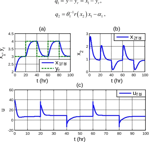
The simulation results for the FBL versus BS designs using the gains reported in Sections 3 and 4 are shown in

Figure 3 and Figure 4 for comparison purposes.

It can be seen that both x_1fbl

( )

t →y t_r

( )

and x_1bs

( )

t →y t_r

( )

asymptotically with no overshoot. It can also be seen that the magnitudes of u_fbl

( )

t are slightly larger than those of u_bs

( )

t . However, the reverse can also be obtained by tuning K_fbl and

{

c c₁, ₂

}

.

6. Observer-Based FBL and BS Controls

[image:7.595.199.426.487.689.2]

As mentioned before that not all state variables are measured in the bioreactor systems; therefore, suitable ob-servers are needed for realizing the full-state feedback control designs proposed in Sections 3 and 4. We shall

Figure 2.Responses of closed-loop bioprocess(41)under BS control ubs

( )

t for c1=c2=8.

0 20 40 60 80 100

1 2 3 4

t (hr)

x 1

, y

r

(a)

x1bs

yr

0 20 40 60 80 100

0 1 2 3

t (hr)

x 2

(b)

x2bs

0 10 20 30 40 50 60 70 80 90 100

-20 0 20 40

t (hr)

u

(c)

[image:8.595.200.425.82.277.2]

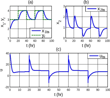
Figure 3. Comparing FBL responses in Figure 1 and BS responses in Figure 2.

Figure 4. Zoomed-in view of x1fbl

( )

t and x1bs

( )

t and

( )

fbl

u t and ubs

( )

t in Figure 3.

investigate the constructions of Luenberger observers for the FBL-based and BS-based control approaches in this section

6.1. Luenberger Observer for FBL Control

Since only x t1

( )

is measured in (4), a Luenberger observer [12] can be constructed for full-state estimation

needed for full-state control of the bioprocess system. Using (21), a full-state observer can be constructed as

(

)

(

)

(

)

(

)

1 1 1 1

ˆ ˆ ˆ ˆ ,

ˆ ˆ ˆ ˆ

, ,

c c fbl c fbl r r o c fbl r r

c c

y y y y y

y z x y z x

 = − + + + − = + + +

 

= = = = = =



 _{ }

z A B K z B K Y L A z B K Y L

C z C z

(42)

where A_o A_c−B K_{c fbl}−LC_c is the observer system matrix and _∈ 2 1×

L  the observer gain matrix to be de-termined such that A_o is Hurwitz, provided that 

(

Ac−B Kc fbl

)

,Cc is an observable pair (which is the case

in the present problem). The gain matrix L in (42) can be computed using a Luenberger observer [12] with pole placement (PP) and/or Kalman-Bucy filter [13] design techniques. We shall focus on the PP design method;

0 20 40 60 80 100

2 2.5 3 3.5 4 4.5

t (hr)

x 1

(a)

x1f bl

x1bs

0 20 40 60 80 100

0 1 2 3 4

t (hr)

x 2

(b)

x2f bl

x2bs

0 10 20 30 40 50 60 70 80 90 100

-20 0 20 40 60

t (hr)

u

(c)

uf bl

ubs

0 5 10 15 20 25 30 35 40 45 50

1 2 3 4

t (hr)

x 1

(a)

x1f bl

x1bs

0 5 10 15 20 25 30 35 40 45 50

-20 0 20 40

t (hr)

u

(b)

[image:8.595.201.426.313.534.2]

henceforth L and A_o=A_c−B K_{c fbl}−LC_c in (42) will be denoted by L=L_pp and A_opp=A_c−B K_{c fbl}−L C_{pp c}, respectively. It should be noted that for a general LTI system characterized by

[

A B C, ,

]

, where

[

A C,

]

is an observable pair, the pair _

(

A−BK

)

,C_ may not be observable, because full-state feedback can destroy ob- servability; furthermore,

(

A BK− −LC

)

may be unstable even though

(

A−LC

)

is designed to be stable [14] [15].

Now using (21) and (42), it can readily be shown that the estimation error z= −z zˆ satisfies, , (0)

opp o

= =

z A z z z , (43) where the initial condition z

( )

0 is arbitrary. Since A_opp is Hurwitz, it follows that

( )

( ) ( )

ˆ

lim lim 0

t→∞z t =t→∞z t −z t = (44)

for all z

( )

0 ≠0.

Using the transformation defined by (17), the observer described by (42) in the

z

-coordinates can be trans-formed back to the x-coordinates as

( )

( )

( )

( )

(

)

1 1

1

ˆ= −_fbl ˆ ˆ= ˆ + ˆ uˆ_fbl+ _fbl− ˆ _pp y−xˆ

x Q x z f x g x Q x L , (45)

where

( )

( )

1

1 _ˆ fbl _ˆ

fbl

−

− ∂ 

 _∂ 

 

T

Q x x

x

 and Q_fbl

( )

xˆ is the Jacobian matrix associated with (17) given by

( )

(

1 1

)

1 2

2

2 ₂

1 0

ˆ ˆ

ˆ

1

ˆ _ˆ

s fbl

s _s

C K x C x

K x _{K x}

 

 

=  ₋ 

 + ₊ 

 

Q x . (46)

In summary, the observer-based control system with feedback linearization for the bioprocess under consider-ation has the form

( ) ( )

uˆfbl,

( )

0 o,

= + =

x f x g x x x (47)

( )

( )

1

( )

(

)

( )

1

ˆ= ˆ + ˆ uˆ_fbl+ −_fbl ˆ _pp y−xˆ , ˆ 0 = ˆ_o

x f x g x Q x L x x , (48)

where xˆ 0

( )

is the initial estimate of x

( )

0 and

( )

( )

1 _{ˆ ˆ}

ˆ_fbl ˆ

u =β− x _−α x +v_, (49)

( )

ˆ

ˆ _{fbl fbl fbl r r}

v= −K T x +K Y +y , (50)

( ) (

)(

)

(

)

(

)

(

)

2

1 2 2 1 1 2 1 1 2 1 2 1 2 1 1 2

2 3 2

2 2 2

ˆ ˆ ˆ ˆ ˆ ˆ ˆ ˆ ˆ ˆ ˆ

ˆ

ˆ ˆ ˆ

s s S S

s s s

C x K x C x x K x x x C C K x x C K x x

K x K x K x

α = − − − − + −

+ + +

x , (51)

( )

1 1

2 2

( )

ˆ . ˆ S

s C K x

K x

β

+

=

x (52)

6.2. Luenberger Observer for BS Control

In this section we pursue our final objective, i.e., to design a Luenberger observer based on the BS formulation using the error Equation (40). To construct an observer for (40), we need an output equation which can be de-fined as,

[

]

1 1 0 q

We present the following proposition.

Proposition 1

Consider the bioprocess system described by (3) and (4). A Luenberger observer for the associated error system (40) with measurement given by (53) can be constructed as

(

)

( )

ˆ= _qˆ+ _bs y− _qˆ , ˆ 0 = ˆ_o,

q A q L  C q q q (54) where y−C q_qˆ= −y xˆ₁ and L_bs∈2 1× is the observer gain matrix to be determined by, for example poleplace- ment, such that the observer matrix A_obs=A_q−L C_bs is Hurwitz. Since A_q is already Hurwitz and A Cq, q

is an observable pair, L_bs can be determined such that the real parts of the eigenvalues of A_obs =A_q−L C_{bs q}

lie on the left-side of those of A_q on the open left-half plane, if desirable. Furthermore, (54) can be expressed in the x-coordinates as

( )

( )

1

(

)

( )

1

ˆ= ˆ + ˆ uˆ_bs+ _bs− _bs y−xˆ , ˆ 0 = ˆ_o.

x f x g x Q L x x (55)

Proof: First, we need to show that the estimate qˆ converges to its true value q. Define the estimation error as q= −q qˆ. From (40) and (54), it follows that q satisfies,

(

)

(

)

( )

ˆ _{q bs q} ˆ _obs , 0 _o,

= − = − − =

     

q q q A L C q q A q q q (56) where q

( )

0 is the initial condition. Since A_obs is Hurwitz, it follows that

[ ]

[

ˆ

]

lim lim 0

t→∞ q =t→∞ q q− = , (57)

for arbitrary q

( )

0 Next, using, (24), (25) and (29), the coordinates transformation for the error-system can be obtained as

( )

1

(

)

( )

(

1

)

1 1

1 2 1 1 1 2 1 1 1 1

, ,

1

r r

bs r r

r r

x y x y

y y

r x x r x x c x c y y

θ− α θ−

− −

   

=_{ } =_{ }

− + − − −

   

q T x 

 . (58)

Equation (58) yields the Jacobian matrix

( )

1

_{( ) (}

₎

1

1 2 1 1 1

2

1 0

1 bs

bs r

r x c x

x

θ− θ−

 

∂ _{ }

=_ ∂ _

+ −

∂

∂

 

 

T

Q x

x

 , (59)

where Q_bs is nonsingular for ₁1 ₁

2

0 r

x x

θ− ∂ _≠

∂ so that Tbs

(

x,y yr,r

)

is a local diffeomorphism for (3). Equa-

tions (58) and (59) yield qˆ=Q_bs

( )

x xˆ ˆ and, from (53) and (54),

( )

( )

(

)

( )

( )

( ) (

)

1 1 1

1 1

ˆ= _bs− ˆ ˆ= _bs− ˆ _ _qˆ+ _bs y−xˆ _= ˆ + ˆ uˆ_bs+ _bs− ˆ _bs y−xˆ

x Q x q Q x A q L f x g x Q x L , (60)

where 1

( )

_ˆ bs −

Q x is the inverse of Q_bs

( )

xˆ , and

( )

1

1

1 1 2 2 1 1

2

ˆ ˆ

ˆ ˆ ˆ ˆ

ˆ bs

r

u x c q q

x

θ φ α

− −

 ∂  _{ }

=_{  }− − − + _

∂

  x

 _{, (61)}

(

)

1

( )

1 1 1 1 1 1 1 2 1 2 1 1 1

ˆ c qˆ xˆ y_r c c qˆ qˆ r xˆ xˆ xˆ y_r, c 0,

α _{= −}  _{+ +}  _{= − − + +}θ− _{− + > (62)}

which complete the proof. 

The observer design technique developed here is interesting and attractive and is different from the two-filter approach in [9]. The technique can be applied to a wide class of BS-based error systems.

In summary, the observer-based control system with the BS formulation for the bioprocess is described by

( ) ( )

uˆ , bs

( )

0 o

= + =

( )

( )

1

( ) (

)

( )

1

ˆ= ˆ + ˆ uˆ_bs+ _bs− ˆ _bs y−xˆ , ˆ 0 = ˆ_o,



x f x g x Q x L x x (64)

where xˆ 0

( )

is the initial estimate of x

( )

0 .

Simulation studies for the proposed observer-based FBL and BS controls were conducted and compared. The initial conditions were chosen as x

( )

0 =

[

2 0.9

]

T and xˆ 0

( )

=

[

0.8 0.1

]

T. The set-point reference y t_r

( )

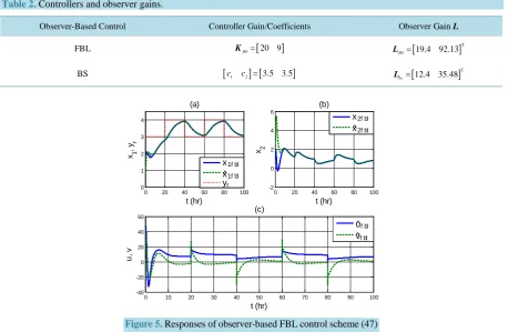
was the same as before. The model parameters were given in Table 1 and Table 2.

In Figure 5,results for observer-based FBL control scheme described by (47) and (48) are shown. It can be seen that the estimates xˆ_1fbl

( )

t →x t₁

( )

and xˆ_2fbl

( )

t →x t₂

( )

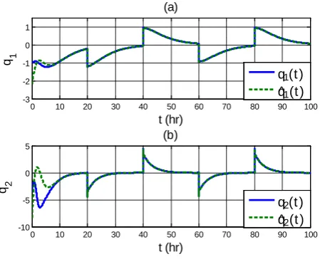
converged to the true states around t=7 h. In

Figure 6, results for the observer-based BS control scheme are presented. Convergence of the estimated states to the actual states can also be seen from this figure, and are similar to those presented inFigure 2.

In Figure 7, the behavior of the error variables q₁ and q₂ defined by (24) and (25) which satisfy (40) in the backstepping scheme is shown. It is evident that q tˆ₁

( )

→q t₁

( )

and q tˆ₂

( )

→q t₂

( )

smoothly after the tran-sients are over around t=8 h.

7. Conclusion

Observers are critical to control system analysis and designs that employ full-state feedback, where not all the state variables are accessible for on-line, real-time measurements, and/or where the measurements are corrupted by noise. Indeed, the design of suitable linear or nonlinear observers or filters leading to observer-based control technology is an integral part of real world control system applications. In this paper, observer-based control strategies were developed for a nonlinear bioprocess system using feedback linearization and backstepping con-trol techniques; in particular, a Luenberger observer for backstepping concon-trol was formulated using the error equation resulted from the backstepping design procedure. The observer design technique developed here is in-teresting and attractive and is different from the two-filter approach known in the literature. Simulation results with and without observers for both the FBL and BS schemes are presented and compared. The results were ex-cellent and demonstrated the feasibility and effectiveness of the proposed approaches.

Table 2. Controllers and observer gains.

Observer-Based Control Controller Gain/Coefficients Observer Gain L

FBL Kfbl=[20 9] [ ]

T

19.4 92.13 fbl=

L

BS [c1 c2] [=3.5 3.5] [ ]

T

12.4 35.48 bs=

[image:11.595.85.544.404.703.2]

L

Figure 5.Responses of observer-based FBL control scheme (47) and (48): xˆ1fbl

( )

t →x t1

( )

and xˆ2fbl

( )

t →x t2

( )

smoothly.

0 20 40 60 80 100 0

1 2 3 4

t (hr) x 1

, y

r

(a)

x1f bl

^ x1f bl

yr

0 20 40 60 80 100 -2

0 2 4 6

t (hr) x2

(b)

x2f bl

^ x2f bl

0 10 20 30 40 50 60 70 80 90 100 -40

-20 0 20 40 60

t (hr)

u

, v

(c)

^ uf bl

[image:12.595.201.425.84.278.2]

Figure 6. Responses of observer-based BS control scheme (63) and (64): xˆ1bs

( )

t →x t1

( )

and xˆ2bs

( )

t →x t2

( )

smoothly.

Figure 7. Evolution of the backstepping error variables:

( )

( )

1 1

ˆ

q t →q t and q tˆ2

( )

→q t2

( )

smoothly.

Acknowledgements

The authors would like to thank all the reviewers for their feedbacks and constructive criticisms.

References

[1] Bastin, G. and Dochain, D. (1990) On-line Estimation and Adaptive Control of Bioreactors. Elsevier, Amsterdam. [2] Dochain, D. (2003) State and Parameter Estimation in Chemical and Biochemical Processes: A Tutorial. Journal of

Process Control, 13, 801-818. http://dx.doi.org/10.1016/S0959-1524(03)00026-X

[3] Dochain, D. and Rapaport, A. (2005) Internal Observers for Biochemical Processes with Uncertain Kinetics and Inputs.

Mathematical Biosciences, 193, 235-253. http://dx.doi.org/10.1016/j.mbs.2004.07.004

[4] Dochain, D. (2000) State Observers for Tubular Reactors with Unknown Kinetics. Journal of Process Control, 10, 259-268. http://dx.doi.org/10.1016/S0959-1524(99)00020-7

[5] Hulhoven, X., Vande Wouwer, A. and Bogaerts, Ph. (2006) Hybrid Extended Luenberger-Asymptotic Observer for Bioprocess State Estimation. Chemical Engineering Science, 61, 7151-7160.

http://dx.doi.org/10.1016/j.ces.2006.06.018

0 20 40 60 80 100 0

1 2 3 4

t (hr)

x1

, y

r

(a)

x1bs

^ x1bs

yr

0 20 40 60 80 100 0

0.5 1 1.5 2 2.5

t (hr)

x2

(b)

x2bs

^ x2bs

0 10 20 30 40 50 60 70 80 90 100 -40

-20 0 20 40 60

t (hr)

u

(c)

^ ubs

0 10 20 30 40 50 60 70 80 90 100 -3

-2 -1 0 1

t (hr)

q 1

(a)

q1(t )

^ q1(t )

0 10 20 30 40 50 60 70 80 90 100 -10

-5 0 5

t (hr)

q 2

(b)

q2(t )

[image:12.595.202.427.321.503.2]

[6] Dochain, D. and Perrier, M. (2003) Adaptive Backstepping Nonlinear Control of Bioprocesses. International Federa-tion of Automatic Control Proceedings, ADCHEM, 77-82.

[7] Khalil, H.K. (2002) Nonlinear Systems. 3rd Edition, Prentice Hall, Upper Saddle River.

[8] Marquez, H.J. (2003) Nonlinear Control Systems: Analysis and Design. John Wiley & Sons, Hoboken.

[9] Krstic, M., Kanellakopoulos, I. and Kokotovic, P. (1995) Nonlinear and Adaptive Control Design. John Wiley, New York.

[10] Isidori, A. (1995) Nonlinear Control Systems. Springer-Verlag, New York. http://dx.doi.org/10.1007/978-1-84628-615-5

[11] Krener, A.J. (1999) Feedback Linearization. In: Baillieul, J. and Willems, J.C., Eds. Mathematical Control Theory, Chapter 3, Springer-Verlag, New York, 66-98.

[12] Luenberger, D.G. (1964) Observing the State of a Linear System. IEEE Transactions on Military Electronics, 8, 74-80. http://dx.doi.org/10.1109/TME.1964.4323124

[13] Kalman, R.E. and Bucy, R.S. (1961) New Results in Linear Filtering and Prediction Theory. Transactions of the ASME,

83D, 429-438.

[14] Ogata, K. (2010) Modern Control Systems. 5th Edition, Prentice Hall, Upper Saddle River.