Los Angeles Classification of Esophagitis using Image
Processing Techniques
Santosh S. Saraf
Research Center, Department of Electronics and
Communications Engg. Gogte Institute of Technology,
Belgaum, Karnataka, INDIA
G. R. Udupi
Vishwanathrao Desphande Rural Institute of Technology
Haliyal, Karnataka, INDIA
Santosh D. Hajare
Department of Gastroenterology K.L.E. Hospital and Research
Center, Belgaum, Karnataka, INDIA
ABSTRACT
Esophagitis is a condition of inflammation of the esophageal mucosa, which is also called as acid reflux disease. The cause maybe be due to slackness of the lower esophageal sphintcer which allows acidic contents of the food from stomach to esophagus. Esophagitis is detected by observing the esophagus by video endoscopy of the Upper Gastro-Intestinal tract. The classification of esophagitis is done by analyzing the images captured during the process of endoscopy. Classification of Esophagitis has many standards , with each standard having its plus and minus. The Los Angeles(LA) Classification deals with precise measurement of the mucosal breaks, for an image processing system to measure the mucosal breaks the position of the camera is to be known. We attempt to classify the Esophagitis using LA Classification without the camera position information using low level image features and classification is performed using a neural network classifier. The results of the classifier are compared with inter and intra observer variability studies.
General Terms :
Medical Diagnosis, Decision Support System
Keywords :
Medical diagnosis, Esophagitis, Image Processing, Neural Network, Classifiers
1
INTRODUCTION
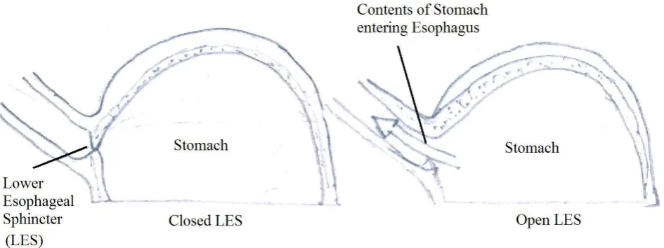
Gastroesophageal reflux disease (GERD) commonly known as acid reflux disease affects nearly 20 % and more people in US and all over the world [1]. It is a condition wherein the contents of stomach escape into the esophagus causing erosion of esophageal mucosa. It manifests as a burning sensation also referred to as heart burn [2]. The cause of heart burn may be due to laxity of the LES (Lower Esophageal Sphintcer) a valve between the stomach and the esophagus fig.1. , which normally does not allow contents of the stomach to escape in the esophagus. The contents of the stomach, which are at a low pH of 1-3, escape into the esophagus with a much higher pH 5-7. This causes inflammation [3,4] and ultimately erosion of the esophageal mucosa which is termed
as Esophagitis. The guidelines for diagnosis of Esophagitis are listed in [5]. Esophagitis maybe due to use of drugs causing reflux or due to lifestyle habits and related causes.[6].
Upper Gastro-Intestinal(GI) Endoscopy can detect Esophagitis. Endoscopy is a process by which the images of the Upper GI Tract covering esophagus, stomach and duodenum are captured. Esophagitis grading is done by observing the esophageal mucosa for the extent of erosion. There are a number of systems for classification of Esophagitis, prominent being Savery Miller classification and Los Angeles Classification. Savery Miller [7] classifies esophagitis into three classes namely Non-Erosive, Erosive and Grade III the description is listed in table 1. Savery Miller method is a broad based classification method which classifies esophagitis into basically two broad classes of erosive or non erosive esophagitis, the severity being dealt in modified Savery Miller method where grade 1, grade 2 and grade 3 classes are included.
Table 1. Savery Miller Classification of Esophagitis Type Description
Non-Erosive Mucosa more towards red side than the normal mucosa.
Erosive Single or multiple erosive regions with confluence
Grade III Circumferential erosive lesions
Los Angeles classification [8] is based on the extent of mucosal breaks and classifies in four grades namely A, B, C and D grades. The details of the grades and the required observation are listed in table 2.
[image:2.595.60.533.89.266.2]
Fig.1 Closed LES and Open LES situation.
[image:2.595.49.286.392.524.2]the mucosal breaks in the radial plane which makes it easy to observe as well as classify [9]
Table 2. Los Angeles Classification of Esophagitis
Type Description
A One (or more) mucosal break 5 mm or less that does not extend between the tops of two mucosal folds
B One (or more) mucosal break more than 5 mm-long that does not extend between the tops of two mucosal folds
C One (or more) mucosal break that is continuous between the tops of two or more mucosal folds but that involves less than 75% of the circumference D One (or more) mucosal break that involves at least
75% of the esophageal circumference
For our study we have considered images in grades B, C, D and normal mucosa, Grade A data was not available because it was felt that Grade A reporting consistency was low [12]. We have implemented neural network based classifier for classification of esophagitis based on LA Classification; the classifier is trained on the low level image features for classification of Esophagitis.
2
MATERIALS AND METHODS
The objective is to measure the amount of erosion of the esophageal mucosa which can be accounted for as texture in the image processing language. The erosion also causes changes in the color wherein a normal mucosa would present itself as salmon pink color and with erosion the color of the mucosa would tend to deep red. Therefore we consider Red,
Green and Blue component images for texture features and Hue, Saturation and Intensity color model to take care of the color changes.
The texture can be seen as changes in intensity of the pixels. The measure of this can be the statistical features of the area of interest. The texture features can be efficiently determined by transforms like Cosine transform and Wavelet transforms. We highlight the features determined for our implementation.
2.1
Statistical Features
The property of texture can be modeled as variation of pixel intensities in a given area. A good measure would be to determine the statistical properties of the variations. The statistical parameters can measure the central tendency and dispersion, the central tendency gives information of location and the dispersion gives information of the spread in the pixel values. We determine the mean (µ) (average) of the image to get the central tendency and the standard deviation (σ)of the image to get the dispersion. The skewness (s) of the data is measured to get the information of the symmetry and kurtosis (k) is determined to get the information of flatness in the values of the pixel. The equations for the statistical parameters are listed in equations (1) – (4).
1. Mean (µ)
mn
n
i
m
j
a
i
j
1
1
,
(1)ai,j is the pixel value of an image of size m x n.
2. Standard Deviation (σ)
mn
p p
a mn 1
2 1
2 / 1
(2)3. Skewness (s)
3mn 1 p 3
1
)
(
s
mn
a
p (3)4. Kurtosis (k)
4mn 1 p 4
1
)
(
k
mn
a
p (4)The four parameters mean (µ), standard deviation (σ), skewness (s) and kurtosis (k) are determined for Red, Green and Blue components of the image.
2.2
Discrete Cosine Transform (DCT)
DCT is a spectral method of determining the texture features[10,11]. The transform helps to decorrelate the local variations in pixels. A two dimensional DCT of an image of size mxn yields matrix of the same size containing the DCT coefficients which give information of the textural tones in the image.
The definition of the two-dimensional DCT for an input image P and output image Q is
10 ,0 1,0 1
1 0 2 1 2 cos 2 1 2 cos M
m p M q N
N n N q n M p m mn P q p pq
Q
(5)
1 1 , 2 0 , 1 M p M p M p
1 1 , 2 0 , 1 N q N q N q
(6)where M and N are the row and column size of P, respectively, Qpq are the DCT coefficients.
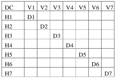
The DCT coefficients for 8x8 size and 64 basis function is shown in figure 2. DC (Q00) is the DC coefficient of the image which indicates the intensity, H, V and D are coefficients indicating the energy in the Horizontal tones of texture, Vertical tones of texture and mixture of both the tone respectively. The vertical tones increase from left to right and the horizontal tones increase from top to bottom, similarly the mixed tones increase diagonally.
The feature set will include the DC coefficient, the mean of the H, V and D components and the energy in each of these components. These features are determined for RGB components of the images
DC V1 V2 V3 V4 V5 V6 V7
H1 D1
H2 D2
H3 D3
H4 D4
H5 D5
H6 D6
H7 D7
Fig. 2. 8x8 DCT matrix, Vi is vertical components, Hi is horizontal components, Di is Diagonal components.
2.3
Discrete Wavelet Transform
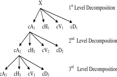
Wavelets form the basis for spatial/scale analysis of images. Discrete Wavelet Transform (DWT) involves scaling and translation process with application of a function – mother wavelet over the image[12,13,14]. The transform decomposes an image in different scale levels, thus from a single image we get multi-scale images and images with horizontal, vertical and diagonal components of the image. Wavelets are functions defined over a finite interval and having an average value of zero. It is based on scaling and translation of the mother wavelet. The process of wavelet transform using filter banks is illustrated in figure 3.
L H 2 2 L H L H 2 2 2 2 X cV cD L H
Low Pass Filter
High Pass Filter
cA
[image:3.595.331.526.70.203.2]cH
Fig. 3 Process of Discrete Wavelet Transform
In figure 3. approximation coefficients matrix cA and details coefficients matrices cH, cV, and cD (horizontal, vertical, and diagonal, respectively) are obtained by wavelet decomposition of the input matrix X. L and H are Lowpass and Highpass filters respectively.
[image:3.595.54.241.72.210.2] [image:3.595.318.550.388.539.2]2.4
Hue Saturation and Intensity Color
Model (HSI)
Three component images RGB images are captured by the process of endoscopy. Since the inflammation and subsequent erosion of the esophageal mucosa results in changes in the color of the esophageal mucosa, to account for the change, using Hue Saturation and Intensity model is appropriate since the Hue and Saturation components give a good measure of the color[15,16]. The HSI model is based on human color perception and useful in cases where illumination varies. Transformation of RGB to HSI allows analysis of all the three components. The equations to determine HSI from RGB is listed in equations (7) to (9)
X
cA
1cH
1cV
1cD
1cA
2cH
2cV
2cD
2cA
3cH
3cV
3cD
31
stLevel Decomposition
2
ndLevel Decomposition
[image:4.595.70.274.237.372.2]3
rdLevel Decomposition
Fig.4 Three level DWT decomposition of the image.
3
)
(
R
G
B
I
(7)
)]
,
,
(
[
)
(
3
1
Min
R
G
B
B
G
R
S
(8)
5
.
0
2
5
.
0
1
cos
B
G
B
R
G
R
B
R
G
R
H
(9)
The mean, standard deviation, skewness, kurtosis and range of the three components Hue, Saturation and Intensity are determined for the image.
2.5
Classifiers
The objective of many image processing and medical systems combined together is to classify a given set of features in known classes. We implement a feed forward neural network for classification. The general process is to determine features and design a classifier to classify the features. Neural Network classifiers work well with n-dimensional feature spaces. The time required from feature determination to classification is improved by packages which allow neural network
phase wherein features are used to train the neural network is slow but once trained they perform well in classification.
The Neural Network structure usually has input layer, hidden layer and the output layer. The input layer contains n number of nodes where n is the number of features. The output layer contains one or m neurons based on the implementation of the network, m being the number of classes. We have implemented feed forward neural network for each set of features. The classifier performance is evaluated by parameters determined by the confusion matrix.
The confusion matrix maps the output of the classifiers as shown in fig.5
True False
True True Positive (TP)
False Negative (FN) False False Positive
(FP)
[image:4.595.55.275.435.582.2]True Negative (TN)
Fig. 5. Confusion Matrix
The mappings are done for a class – True Positive (TP) are the number of samples classified correctly as belonging to the class, False Positive (FP) are the number of samples mapped as belonging to the said class though they do not belong to the class, False Negative (FN) are the number of samples reported as belonging to other class than itself. True Negative (TN) is the number of samples correctly classified as belonging to other class.
1. Precision (P) : Percentage of positive predictions that are correct
%
100
)
(
TP
FP
x
TP
P
(10)2. Sensitivity (Se): The percentage of positive labeled instances that were placed
as positive.
%
100
)
(
TP
FN
x
TP
e
S
(11)3. Specificity (Sp): The percentage of negative labeled instances that were predicted as negative.
100
%
)
(
TN
FP
x
TN
p
S
(12)4. Accuracy (A): The percentage predictions that were correct.
100
%
)
(
)
(
x
FN
FP
TN
TP
TN
TP
A
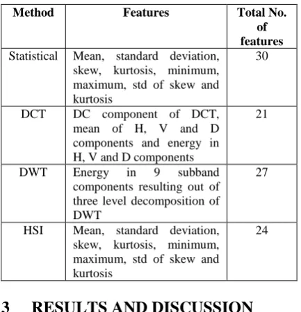
being normal mucosa images. Fifty images per class with a size of 224 x 224 pixels were selected. We have determined features with four methods namely Statistical, DCT, DWT and HSI and trained feedforward neural networks for classification in each case. The details of features selected and the results are listed in table 3 and table 4 respectively.
Table 3. Details of method used to determine features , features and total number of features used to train classifiers.
Method Features Total No. of features
Statistical Mean, standard deviation, skew, kurtosis, minimum, maximum, std of skew and kurtosis
30
DCT DC component of DCT, mean of H, V and D components and energy in H, V and D components
21
DWT Energy in 9 subband components resulting out of three level decomposition of DWT
27
HSI Mean, standard deviation, skew, kurtosis, minimum, maximum, std of skew and kurtosis
24
3
RESULTS AND DISCUSSION
Neural Network classifiers were trained for each method using back propagation algorithm. The Sensitivity and Specificity results in each case are listed in table 4
The results indicate the sensitivity for Normal and Class D is good ranging from 90% - 100% indicating that the whole image analysis gives a good feature space separation and thus a good classification efficiency for the extreme cases. The sensitivity for Class C and Class B are in the range of 50% to 65 % with Class C having better sensitivity compared to Class B. Statistical, DCT and DWT parameters have good overall efficiency in the range of 74% to 76% compared to HSI parameters. The kappa values vary between 0.683 to 0.6
LA Classification by presenting images and video to experts and trainee gastroenterologists has been reported in [17-22]. The kappa for intra-observer agreement was 0.54 and inter-observer agreement was 0.22 reported by [17]. The following literature [18] conducted study of inter-observer variability by presenting both video and still images kappa value was 0.4. [19] and [20] found moderate inter-observer variability. It was found that inter-observer variability is better among
[image:5.595.53.270.176.401.2]trainees [17]. They could report Grade A more accuracy than experts.
Table 4. Sensitivity and Specificity of Neural Network Classifier for various feature sets.
4
CONCLUSION
Although the LA classification is precise in its specifications for classification, for an image captured without the knowing the location of the camera and the esophageal mucosa distance, it is difficult to get a good measure of the mucosal break. Using whole image analysis gives satisfactory results for mucosal breaks above class C which manifests itself as texture information in the image. As reported in the discussion the moderate kappa values for inter and intra observer variability supports our approach of whole image analysis with significant results without considering the Grade A class.
The image segmentation approach meets with a hurdle of detection of precise Z line to determine the end of esophagus to the beginning of stomach which significantly contributes to erosion detection. Precise measurements are possible with image segmentation method with additional information of the distance between the camera and the esophageal mucosa.
Feature
Set Class
Sensitivity (Se) x
100%
Specificity (Sp) x
100%
Overall Efficiency
& Kappa
Statistical Parameters
Normal 0.90 0.90
76% 0.683
Class B 0.55 0.96
Class C 0.60 0.98
Class D 1.00 0.79
DCT Parameters
Normal 0.95 0.91
75% 0.667
Class B 0.50 0.98
Class C 0.65 0.96
Class D 0.90 0.76
DWT Parameters
Normal 0.95 0.95
74% 0.65
Class B 0.60 0.98
Class C 0.50 0.98
Class D 0.90 0.71
HSI Parameters
Normal 1.00 0.92
70% 0.6
Class B 0.50 1.00
Class C 0.50 0.90
REFERENCES
[1] Source : National Digestive Diseases, Information Clearinghouse(NDDIC)
(http://digestive.niddk.nih.gov/statistics/statistics.aspx#sp ecific)
[2] Fass, R, Tougas G.,Functional heartburn: the stimulus, the pain, and the brain, Gut, 2002;51: 885-892
[3] Hungin, A P. S, Raghunath, A. S, Wiklund, I., Beyond heartburn: A Systematic review of the extra-oesophageal spectrum of reflux-induced disease. Fam Pract., 2005; 22: 591-603
[4] Kaltenbach, T., Crockett, S., Gerson, L. B. , Are lifestyle measures effective In patients with gastroesophageal reflux disease?: an evidence-based approach, Arch. Intern Med,2006; 166: 965-971
[5] DeVault KR, Castell DO.,Guidelines for the diagnosis and treatment of gastroesophageal reflux disease. Arch Intern Med 1995;155:2165–73
[6] Tefera L, Fein M, Ritter MP, et al., Can the combination of symptoms and endoscopy confirm the presence of gastroesophageal reflux disease?, Arch. Surg, 1997;63:933– 6.
[7] Savary M, Miller G. The Esophagus. Handbook and Atlas of Endoscopy. Solothurn: Gassmann Verlag, AG, 1978.
[8] Lundell L, Dent J, Bennett J, et al. Endoscopic assessment of esophagitis: clinical and functional correlates and further validation of Los Angeles classification. Gut 1999; 45:172-80
[9] Tomoko Katsube, et. al., Difference in Localization of Esophageal Mucosal Breaks Among Grades of Esophagitis Posted: 01/16/2007; Journal Gastroenterol Hepatol. 2006;21(11):1656-1659. © 2006 Blackwell Publishing
[10]G. Sorwar, A. Abraham and L. Dooley, “Texture Classification Based on DCT and Soft Computing”, in the 10th IEEE International Conference on Fuzzy Systems, Melbourne, Australia, December 2001. [11]Image Segmentation Using Discrete Cosine Texture
Feature Chi-Man Pun and Hong-Min Zhu, International Journal of Computers,Issue 1, Volume 4, 2010, 19-26
[12]G. Menegaz, “DWT-based non-parametric texture modeling,” in Proc. of the International Conference on Image Processing (ICIP), 1, pp. 173–176, 2001.
[13]Chang, T., Jay Kuo, C.C., 1993. Texture analysis and classification with tree-structured wavelet transform. IEEE Trans. Image Process. 2 (4), 429–440
[14]Arivazhagan, S., Ganesan, L., 2003. Texture classification using wavelet transform.Pattern Recogn. Lett. 24 (9–10), 1513–1521
[15]Cheng, H. D. Jiang, X. H. Sun, Y. Wang, J., Color image segmentation: Advances and prospects Fitting, PATTERN RECOGNITION, 001, VOL 34; PART 12, pages 2259-2282,
[16]H. D. Cheng, X. H. Jiang, and Y. Sun, A Survey on Color Image Segmentation,” The First International Workshop on CVPRIP, Triangle Park, North Carolina, 1998.
[17] Siavosh Nasseri-Moghaddam, et. al., Inter- and Intra-Observer Variability of the Los Angeles Classification : A Reassessment, Archives of Iranian Medicine, Vol. 10, No.,1, Jan.,2007, 48-53.
[18]Armstrong D, et.al., The endoscopic assessment of esophgatis : a progress report on observer agreement, Gastroenterlogy, 1996, III:85-92
[19]Pandolfino J.E., Vakil N.B., Kahrilas P J, Comparison of inter- and intra-observer consistency for grading of Esophagitis by expert and trainee endocopist, Gatrointest Endosc., 2002, 56:639-643.
[20]Rath HC, et. al. , Comparison of inter-observer agreement for different Scoring systems for reflux esophgatis: impact of level of experience, Gastrointest Endosc., 2004;60:44-49.
[21]Kusano M, et.al., Inter-observer variation in endoscopic assessment of GRED using the Los Angeles classification, Gastrointest Endosc., 1999;49:700-704. [22]Bytzer P, et. al., Inter-observer variation in the