Joint State and Parameter Estimation of Squirrel Cage
Induction Motor – A System Identification Approach using
EM based Extended Kalman Filter
K.Radhakrishnan
M.A. College of EngineeringKothamangalam Kerala, India
A.Unnikrishnan
NPOLKochi Kerala, India
K.G.Balakrishnan
CUSATKochi Kerala,India
ABSTRACT
This paper deals with the recursive optimum estimation of rotor resistance, inductance and stator resistance of induction motor. The estimation of parameter and states in the presence of system noise is achieved using EKF, which takes in to account measurement and modelling inaccuracies. A major limitation in the parameter estimation using EKF is that its optimality is dependent on the choice of the right covariance matrices. In this paper the EM(Expectation Maximization) algorithm along with the Kalman smoothing is used to obtain the initial values of process and measurement covariance matrices. The Vas model of the induction motor is used for simulation and the rotor inductance, rotor resistance and stator resistance are considered as parameters as well as states. For the estimation of these parameters, the state vector is augmented with these parameters to be estimated. The parameters used for simulation is that of a three phase, 2.2 kw, 400V, 50 Hz cage induction motor. Matlab is used to simulate the system and from the results it is observed that the parameter estimates converges to true values with a reasonable degree of accuracy.
General Terms
Parameter estimation, System Identification, Expectation Maximisation
Keywords
Kalman filter, Induction motor.
1.
INTRODUCTION
Induction motors are widely used in industry since they are very economical, rugged and reliable, and are available in wide ranges of capacity. Unlike D.C motors, they have highly non-linear characteristic, requiring more complex control algorithms. When variable speed is required the D.C machines are the most suitable electromechanical devices, as they have the advantage of precise speed control when utilized for the purpose of accurate driving. On the other hand induction motors are robust, simple, small in size, low in cost and almost maintenance free [1][2]. The main obstacle in using induction motor drives is high cost of conversion equipment, the complexity of signal processing and poor precision in achieving effective speed and torque control. Speed control with a dynamic performance similar to that of a D.C motor can be achieved using field-oriented control(FOC), which requires an estimate of the rotor
flux. In the estimation of the rotor flux, the knowledge of the machine parameter and in particular the rotor time constant (TR=LR/RR) is needed. However the electric parameters may deviate from the original values due to changes in the working environment, temperature, speed, external load and noise. The inaccurate knowledge and parameter variation can deteriorate the achieved control and performance of the motor. Thus it becomes necessary to estimate the real time parameters. In this paper the values of Rs,Rr,Lr are estimated using the EKF and the measurement of the stator currents and voltages.
The ability of the extended Kalman filter[3]-[8] to simultaneously estimate the states and the parameters of a dynamic system is well known. It allows for the real evaluation of the parameter uncertainties and errors due to the model simplification. A Kalman filter estimates the states of a dynamic system with two different models namely the process model and the observation model. The dynamic model describes the behaviour of the different dynamic states while the observation model establishes the relationship between the measurement and the state vector. Both models are associated with the statistical properties to describe the accuracy of the models. It uses the underlying process model to make an estimate of a system and corrects the estimate using available sensor measurements. Using this predictor corrector mechanism, it approximates an optimal estimate due to linearisation of the process and measurement models.
The Kalman estimator is based on the assumption of known apriori statistics to describe the measurement and process noise[9]-[10]. The tuning of the covariance matrices of them is done manually in many EKF implementations, a major draw- back of it for the parameter estimation. Moreover the matrices of parameter governing the transformations in the measurements and process equations are typically unknown. The optimality of Kalman filter often depends on the formation of these apriori. These limitations in estimating these noise co variances are overcome using EM algorithm[11]-[12].
2.
THE INDUCTION MOTOR MODEL
The model of the induction motor used is the Vas model deduced from the park transform[2]. This model considers the stator voltages U=[Usα Usβ]T as input and the stator currents Y=[Isα Isβ]T as output. The stator currents and rotor flux arechosen as the state variables: X=[Isα IsβψRαψrβ]T. The fourth order model in the mechanical frame is given by the following equations.
=
)
(
t
X
&
A X(t) + B U(t) (1) Y(t) = C X(t) (2) where[
]
[
]
= =
− − −
− − −
=
= =
C T
L K L K B
R T R
T H L
R T R
T H L
L K R L
R R H L L K R L
H L L K
R K
L K R L
H L L K R L
R R H L L
K R K
A
T s u s u U T R R is is X
0 0 1 0
0 0 0 1
1 0
1 0
2 0
2 0
ω
ω ϖ
ϖ β α β
ψ α ψ β α
R R R L
H L S R R K
2 2
+ =
R L
H L Ls KL
2
− =
R R
R L R
T =
where
RS = stator resistance RR = rotor resistance LS = stator inductance LR = rotor inductance LH = magnetizing inductance
i sα, i sβ - components of stator current space vector U sα, U sβ - components of stator voltage space vector
ψRα , ψRβ -components of rotor flux space vector
ω - angular speed of rotor
The discrete time versions are given by the following formulae.
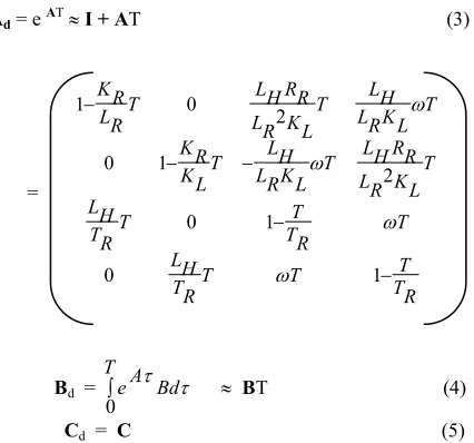
Ad = e AT≈I + AT (3)
=
R T
T T
T R T
H L
T R
T T T
R T
H L
T L K R L
R R H L T L K R L
H L T L K
R K
T L K R L
H L T L K R L
R R H L T
R L
R K
− −
− −
−
1 0
1 0
2 1
0
2 0
1
ω
ω ω
ω
Bd = ∫ T
Bd A e 0
τ τ
≈ BT (4) Cd = C (5) where Ad, Bd, Cd represents the discretised versions of A, B and C. For computation of Ad and Bd, the second order term is neglected. To estimate the parameters, the parameter vector is chosen as
θ(k) =[RS RR NR] (6) Where NR=1/LR.
3.
THE EXTENDED KALMAN
FILTER
ALGORITHM
The conventional type of estimator is a Kalman filter. The model of the Kalman filter is as shown in fig 1. One of the parts of the Kalman filter is a single step extrapolator based on system model. This extrapolator predicts the state variable vector X. The measurement model then transforms the prediction of the estimator to the prediction of the measurement. This prediction is compared with the real measured values. The obtained difference is then used to correct the actual prediction of the estimator.
Y k Xk,k ˆ
Y kˆ
, 1 ˆ
−
k k X
[image:2.612.329.542.90.289.2]U
kFig.1 Model of Kalman filter
K k kk
Ak Ck
For nonlinear systems( in this case induction motor) , the extended Kalman filter has to be used. The EKF is a sophisticated algorithm that is suitable for estimation of the motor parameters and the rotor flux components. To apply the EKF for simultaneous state and parameter estimation, the state vector is augmented by the parameter vector. : Xe(k) = [X(k)
θ(k)] which makes the system non-linear. The new discretized state equations are
) ( )] ( ), ( [ ) 1
(k f Xe k U k We k e
X + = + (7)
Y(k) =h[Xe(k),U(k)]+Ve(k) (8) where Xe(k) ,U(k) and y(k) are the augmented state vector, input vector and output vector. We(k) and Ve(k) are the system and measurement noises respectively. These noises are white with zero mean and characterized by
) ( )} ( ) ( { , 0 )} (
{We k E We kWeT k Q k
E = = (9)
E{Ve(k)}= 0,E{Ve(k)VeT(k)}= R(k) (10) The process covariance matrix Q(k) and measurement covariance matrix R(k) are symmetric and semi-definite. The discrete Kalman filter algorithm [13][14] is as follows.
Prediction ) ( ) ( ) , ( ) ( ) , 1 ( )) , ( ˆ ), , ( ˆ ( ) , 1 ( ˆ k Qe T k F k k Pe k F k k pe k k k k e X f k k e X + = + = + θ (11)
Where Xˆ is the state estimate and
e
Pe is the estimation error covariance and ) , ( ˆ ) ( )) ( ), ( ( ) ( k k e X k Xe k k X f Xe k F = ∂ ∂ = θ Updating )] , 1 ( ˆ ), 1 ( 1 ( [ ) 1 ( ) , 1 ( ˆ ) 1 , 1 ( ˆ k k e X k H k Y S S k K k k e X k k e X + + − + = + + + = + + (12) ) , 1 ( ) 1 ( ) 1 ( ) , 1 ( ) 1 , 1(k k Pe k k K k H k Pe k k
Pe + + = + − + + +
) , 1 ( ˆ ) ( )] 1 , 1 ( [ ) 1 ( k k e X k Xe k k Xe h Xe k H Where + = + + ∂ ∂ = +
The main difficulty of Kalman filter is arriving at the right covariance matrices because for many cases , the required statistical information is not available. This difficulty is overcome using Expectation Maximization (EM) algorithm which is actually a Kalman smoother.
4.
THE EM ALGORITHM
Since the EKF is a sub optimal estimator based on linearisation of a non-linear mapping, X is only an approximation to the expected value and Pk is an approximation to the covariance matrix. Smoothing often entails forward and backward filtering over a segment of data so as to obtain improved averaged estimates. After computing the forward estimates X(k) and
P(k) with EKF, over a segment of N samples, the Rauch – Tung- Stribel smoother[15] is used which makes use of the following backward recursions.
J(k−1)= P(k−1)ATP−1(k,k−1) (13) )] 1 ( ˆ ) ( ˆ )[ 1 ( ) 1 ( ˆ ) 1 (
ˆ k− N = X k− J k− X kN −AX k−
X (14 S k J k P N k
P( −1 ) = ( −1)+ ( −1)
(15)
) 1 ( )] 1 , ( ) ( [ − − −
= P kN P k k JT k
S where 1 ) ( ) 1 ( ) ( ) 1 ,
(k k N P k JT k J k S
P − = − + (16)
) 1 ( )] ( ( , 1 ( [
1= P k+ kN− A P k JT k− S
where
Initialized as follows: ) ( ˆ ) (
ˆ NN X N
X = , P(N N)= P(N) and
) 1 ( ] ) ( ) ( [ ) 1 ,
(N N − N = I −K N GT N AP N−
P
The EKF algorithm for state estimation suffers from serious shortcomings, namely choosing the initial states and covariance. The EM algorithm can be used to obtain the initial values { R ,
Q }. The EM algorithm is an iterative method for finding a mode of the likelihood function p(Yθ ). It can be shown that maximizing E [ln p(X,Yθ ) will ensure an increase in the log-likelihood function, where Y denotes the N measurements { y1, ….yN} and X denotes {X1,……,XN}. The expectation involves averaging over X under the distribution p(XY, θold ) wherein
θold
represents the current estimates of the parameters.
We assume the likelihood of the data given the states, initial conditions and evolutions of the states to be represented by gaussian distributions. Under the initial model assumptions of uncorrelated noises and Gauss – markov state equations, the likelihood of the complete data is given by :
L X p Y X
p( , θ) = ( (1)
(17)
∏ = − ∏= = N k N
k pY k X k
k X k X p L where
2 ( ( ) ( 1)) 1 ( ( ) ( )
Hence, for gaussian approximations, the log-likelihood of the complete data is given by the following expression:
=
) , ( lnp X Yθ
))}] ( ˆ ) ( {( 1 ))} ( ˆ ) ( {( 1 2
1
[ Y k Y k TR Y k Y k N
k −
− −
∑ = −
)}] 1 ( ) ( { 1 } ) 1 ( ) ( { 2 1
2[ − −
− − − ∑
− X k AX k T Q X k AX k
N
) 2 ln( 2
) ( ) ) 1 ( ( 1 ) ) 1 ( ( 2 1
π µ
µ T X N m q
X − Π− − − +
−
Π − − −
− ln
2 1 ln 2
1 ln
2
Q N R N
(18) where Yˆ(k)=h(X(k),U(k))
to implement the EM algorithm for nonlinear state space models, we need to compute the expectation of ln p(X,) and then differentiate the result with respect to the parameters so as to maximize it. The EM algorithm for nonlinear state space model thus involve computing the expected values of the states and covariance with the extended Kalman smoother and then maximizing the parameter with the following formulae obtained by differentiating the expected log- likelihood:
1
− ∆ =γ
A , ( 1 )
1
1 T
N
Q= − Γ−γ∆− γ , µ= Xˆ(1N),
) 1 ( N P
=
Π and ∑
= +
= N
k
T MM k H N k P k T H N R
1 ( ) ( , ) ( ) 1
))} ( ) ( ( ) (
{Y k h X kN U k M
where
− =
) (
2 ( )
ˆ ) (
ˆ P kN
N
k kN
T X N k
X +
∑ = = Γ
) 1 ( ) 1 ( ˆ 2 ( 1 )
ˆ XT k N P k N
N
k∑= X k− N − + −
=
∆ and
) 1 , (
2 ( 1 )
ˆ ) (
ˆ P k k N
N
k k N
T X N k
X + −
∑
= −
= γ
5.
SIMULATIONS AND RESULTS
Simulation using Matlab has been carried out using the experimental data (stator currents and voltages) obtained for a 400 Volts, 50 Hz, 2.2 kw cage induction motor. The state variables are X=[Isα, Isβ, ψrα, ψrβ]
T
.The state vector is augmented with the parameter vector[Rr Rs Lr]to form the new state vector. The rotor resistance, stator resistance and rotor inductance are these parameters. The variations of the estimated parameters are accounted by tuning the parameter components of the covariance matrix Qe. The first four components of the process noise vector We are related to the stator currents and rotor flux. The last three components characterise the parameters’ variations and permit to tune the dynamics of the parameters. The measured voltages are assumed to be uncorrelated. The
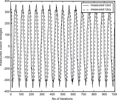
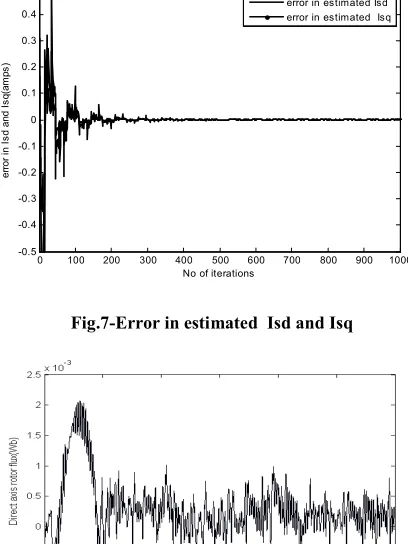
excitation signals for the EKF are the output of a PWM voltage source inverter used to drive the motor at variable speed. In this paper the tuning of Qe and Re is done using the EM method, a major change from the conventional EKF, which uses manual tuning. The initial covariance matrix of Qe and Re obtained by EM method are Qe = diag[ 0 0 2.0707 2.0707 2.0707 2.0707 2.0707 2.0707 ] and Re= [ 2.0322 0.9885 ; 0.9855 2.0102]. Figures 2 and 3 show the measured stator voltages and currents respectively. Figure 4 demonstrates the convergence of estimated parameters. It is seen that Rs, Rr and Lr converges very close to the true values. The error in the convergence of these parameters are shown in figure 5. The mean of these estimated parameters and the variances of the error are given in table1. Figures 6 and 7 demonstrates the estimated direct axis and quadrature axis stator currents and the error in the estimations respectively. Figure 8a and 8b illustrates the estimated direct axis and quadrature axis rotor flux.
0 100 200 300 400 500 600 700 800 900 1000 -400
-300 -200 -100 0 100 200 300 400
m
e
a
s
u
re
d
s
ta
to
r
vo
lt
a
g
e
s
No.of iterations
[image:4.612.343.533.276.439.2]measured Usd measured Usq
Fig.2-Measured stator voltages Usd and Usq
0 100 200 300 400 500 600 700 800 900 1000 -4
-3 -2 -1 0 1 2 3 4
m
e
a
s
u
re
d
s
ta
to
r
c
u
rr
e
n
ts
No.of iterations
[image:4.612.351.530.479.625.2]m easured Is d m easured Is q
0 100 200 300 400 500 600 700 800 900 1000 -4
-3 -2 -1 0 1 2 3 4
No of iterations
Is
d
,
Is
q
(
A
m
p
s
)
[image:5.612.69.262.80.236.2]direct axis stator current Isd quadrature axis stator current Isq
Fig 4 –Estimated Direct and quadrature axis Stator Currents
0 100 200 300 400 500 600 700 800 900 1000 -5
0 5 10
No of iterations
R
r,
L
r,
R
s
(
o
h
m
s
)
[image:5.612.335.539.90.362.2]rotor resistance Rr rotor inductance Lr stator resistance Rs
Fig.5-Estimated parameters Rs , Rr and Lr
0 100 200 300 400 500 600 700 800 900 1000 -3
-2 -1 0 1 2 3
No of iterations
e
rr
o
r
in
R
s
,R
r,
L
r
(o
h
m
s
)
error in Rr error in Lr error in Rs
Fig.6-Error in estimated parameters Rs , Rr and Lr
0 100 200 300 400 500 600 700 800 900 1000 -0.5
-0.4 -0.3 -0.2 -0.1 0 0.1 0.2 0.3 0.4 0.5
No of iterations
e
rr
o
r
in
I
s
d
a
n
d
I
s
q
(a
m
p
s
)
error in estimated Isd error in estimated Isq
Fig.7-Error in estimated Isd and Isq
[image:5.612.340.533.436.570.2]Fig8a- Estimated Direct axis Rotor Flux
Fig.8b-Estimated quadrature axis rotor flux
Table 1 estimated and true values of the
parameters and their variances
Estimated (mean)
True Variamce Rr 2.71139 Ohms 2.72 Ohms 0.00147 Rs 6.36457 Ohms 6.12 Ohms 0.13170 Lr 497.8 mH 418.18 mH 0.96351 Time
constant
[image:5.612.74.265.484.640.2]6.
CONCLUSION
In this paper we have estimated the stator currents, rotor flux, rotor resistance and rotor inductance and stator resistance of a 400 Volts, 50 Hz, 2.2 KW squirrel cage induction motor using fourth order model of the induction motor and EKF. The initial values of Qe and Re were estimated using the EM algorithm. Simulation results show the ability of the EKF along with the EM algorithm to track the rotor flux and the electrical parameters to a reasonable degree of accuracy.
Different internal faults(e.g. partially broken rotor bars, partially broken end rings) can occur due to ageing and due to the environmental conditions under which the machine operate. These faults may cause gradual deterioration of the motor, which may lead to failure of the motor. The estimation procedure adapted in this paper can further be used for early detection of faults, by continuously monitoring the machine parameters. This will reduce the machine down time and enhance the reliability in critical application
7.
REFERENCES
[1] R.Krishnan, Electric Motor Drives ( Pearson Education, Singapore, 2003).
[2] P.Vas, Vector Control of AC Machines ( Oxford University Press, New York, 1994).
[3] K. Radhakrishnan, A. Unnikrishnan and K.G. Balakrishnan, Model Recognition for Estimation of Direction of Arrival using Extended Kalman Filter, Proceedings of the Third IASTED International Conference on Signal Processing , Pattern Recognition, and Applications (SPPRA), February 2006,
[4] M.A. Ouhrouche, EKF Based On-line Tuning of Rotor Time Constant in an Induction Motor Vector Control, International Journal of Power and Energy Systems, 20(2), 2003, 103-110.
[5] L.Salvatore, S.Stasi, and L.Tarchioni, A New EKF Based Algorithm for Flux Estimation in Induction Machines,
IEEE Transactions on Industrial Electronics, 40(5),1997,496-504.
[6] S.Wade, M.W. Dunnigan and B.W. Williams, Modeling and Simulation of Induction Machine Vector Control with Rotor resistance Identification, IEEE Transactions on Power Electronics, 121(3), 1997,495-506.
[7] L.C. Zai, C.L. Demacro, and T.A.Lipo, An Extended Kalman Filter Approach to Rotor Time Constant Measurement in PWM Induction Motor Drives , IEEE Transactions on Industry Applications, 28(1), 1992,96-104. [8] R.E.Kalman, R.S.Bucy, New Results in Linear Filtering and
Prediction Theory, Journal of Basic Engineering, 1961,95-108.
[9] C.K.Chui and Chen, Kalman Filtering with Real Time Applications, Springer Verlag, New York,1991,108-118 [10] A.H. Jaswinski, Stochastic Processes and Filtering Theory,
Academic Press,1970.
[11]A.P. Dempster, N.M Laird and D.B Rubin, Maximum Likelihood from Incomplete Data via the EM Algorithm , Journal of the Royal Statistical Society Series, B 39,1977,1-38.
[12] V.Digalakis, J.R. Rohlicek, M.Ostendorf, ML Estimation of Stochastic Linear System with EM Algorithm and its Application to Speech Recognition, IEEE Transactions on Speech and Audio Processing , 1, 1993,431-442.
[13] Shan-Shu Xiong, Zaho- Yug, Neural Filtering of Coloured Noise Based on Kalman Filter Structure, IEEE Transaction on Instrumentation and Measurement, 52, 2003,742-747.
[14] Roberto Togneri, Li Deng, Joint State and Parameter Estimation for Target Directed Non-Linear Dynamic System Model, IEEE transaction on Signal Processing, 51, 2003,3061-3070.