Enhanced DAGitizer for Grid Computing through the Discovery of Least Cost Path

Enhanced DAGitizer for Grid Computing through the

Discovery of Least Cost Path

D. I. George Amalarethinam,

Department of Computer Science, Jamal Mohamed College, Trichirappalli, Tamil Nadu, India

P. Muthulakshmi

Department of Computer Science SRM University

Chennai, Tamil Nadu, India

ABSTRACT

The need for scheduling algorithms arise from the requirement to perform multitasking, essentially for modern computing systems. Scheduling is the greatest cause that optimizes the objective function that involved with the selection of resources. In scheduling, every aspect of execution is based on decision(s). The general objective of scheduling algorithms is to effectively use the available processors to execute parallel programs, possibly in the least utilization of time. A group of interdependent jobs/tasks forms the workflow application. Scheduling is to map the jobs/tasks on to the collection of heterogeneous resources available in a massive geographic spread. Most complicated applications consist of interdependent jobs that coordinate to solve a problem. The completion of a particular job is the criterion function that has to be essentially met in order to start the execution of those jobs that depend upon it [1]. This kind of workflow application may be represented in the form of a Directed Acyclic Graph (DAG). Grid Workflow is such an application and is modeled by DAG. DAGitizer could generate DAG in a random fashion [2]. This paper proposes a tool (developed using Java) which is an enhanced form of DAGitizer that could find the least cost path between source and destination nodes.

Keywords:

Graph, Randomizer, Communication Cost, Computation Cost, Cost Matrix, Least Cost Path.

1. INTRODUCTION

Grid computing environments are naturally dynamic and random environments that enable sharing of services among numerous, diverse users in wider geographic stretch. Grid schedulers intend to make the most efficient use of Grid resources that could provide best performances to the associated applications. Grid is a collection of resources, which includes networks, machines, applications and data store. Furthermore, grid computing enables careful selection, sharing, coordination of resources; also the integration among the resources. The aim of such computing technology will be met only when the resources are effectively allocated with appropriate jobs. High performance will be achieved only when the scheduling of group of dependent tasks is intensively done. In grids, users may face hundreds of thousands of computers that are available for utilization. Though it is, it is impossible for anyone to manually assign jobs to computing resources in grids. And that an automated means of assigning must be done, which is here meant as scheduling. An effective scheduling aims at minimum turnaround time. To show such scheduling through an illustration, the best ever known possibility is Directed

Acyclic Graph. Grid Workflow scheduling is replicated through Directed Acyclic Graph, and the paper focuses on the generation of effective DAG, which is made in a much automated way through randomizer based on the number of tasks involved[1] and finding the least cost path between an arbitrary source node and an arbitrary destination node.

A directed acyclic graph is a directed graph with no cycles and is formed by a collection of vertices and directed edges, each edge connecting one vertex to another, such that there is

no way to start at some vertex v and follow a sequence of

edges, that eventually loops back to v again[3][4][5].

Scheduling decisions in dynamic scheduling algorithms are made at run time [6]. The objective of dynamic scheduling algorithms include not only creating high quality task schedules, but also minimizing the run time scheduling overheads [7] [8]. The proposed tool generates arbitrary DAGs with a required number of tasks and finds the least cost path between the source and destination nodes, which can be used as test bed to conduct experiments on task scheduling algorithms.

2. RELATED WORKS

The idea of developing a tool that could generate a DAG had been derived by (i) PYRROS, a tool developed by Yang and Gerasoulis [9] is a compile time scheduling and a code generator, which is consisted with a task graph language with an interface to C language. The tool could use only a particular algorithm and is not exclusively a DAG generator; (ii) The application specification tool in PARSA (software developed for automatic scheduling and partitioning of sequential user programs) is accepted with a sequential program written in the SISAL functional language and converted into a DAG and is represented in textual form by an acyclic graphical language called IF1(Intermediate Form 1) [10]; (iii) The idea proposed by Y. K. Kwok and I. Ahmad [11] under scheduling arbitrary DAGs without communication stated that nodes in the DAG can be assigned priorities randomly; (iv) The node and edge weights are usually obtained by estimation at compile time.[12]; (v) Hu’s Algorithm [13] for Tree Structured DAGs, where in-tree structured DAGs had been proposed with unit computations and without communications and the number of processors is assumed to be limited; (vi) Multistage graph problem solved using the technique of Dynamic Programming [14].

3. ARCHITECTURE AND BEHAVIOR

OF THE TOOL

1. Selector 2. Fragmentor 3. Plotter 4. Filter 5. Ascriber 6. Evaluator 7. Tracker 8. Petiter 9. Finalizer

3.1 Architecture of the Tool

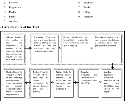
Figure 1. Architecture of enhanced DAGitizer

3.1.1 Selector

This block expects the inputs to be given and thereby it starts functioning. The inputs to be given are (i) number of tasks

(nv) to be in the DAG, (ii) the maximum

COMPCost(MaxCOMPCost), (iii) the maximum

COMMCost(MaxCOMMCost).

The choice of choosing a DAG to be generated is revised to get either (i) DAG with one vertex each in its first and last level or (ii) any number of nodes irrespective of levels

3.1.2 Fragmentor

The Height Factor (HF) is generated by the tool which defines the number of levels to which the DAG has to distribute the tasks (nodes). This can be defined by the user also. If the user defines it, the priority is to user’s choice of height factor.

3.1.3 Plotter

Random assignment of number of successors of each node is done in this block. Each node is identified in a particular level

as vij, where’ vij’ is the vertex at level ‘ i’ and ‘j’ is the

position of the node in the particular level;1≤j≤(number of nodes in level ‘i’). The tool is carefully devised in such a way that the nodes of last level cannot have successor. Similarly there cannot be any parent for the node(s) at the first level.

3.1.4 Filter

As successors are assigned randomly, there might be a possibility of getting more than one link between the same child and parent. This block eliminates duplicates and ensures only one link between a pair of nodes/tasks at different levels.

3.1.5 Ascriber

The summation of COMPCost (TCOMPCost) of all

nodes/tasks and the summation of COMMCost

(TCOMMCost) of all edges are calculated.

3.1.6 Evaluator

The Communication - Computation Ratio (CCR) is calculated in this block and is defined as the ratio between the average communication cost of all the edges and the average computation cost of the nodes.

And can be shown as,

CCR=Average(∑COMMCost(ei)) / Average(∑COMPCost(vj)) ;

1≤i≤nv, 1≤j≤ne (1)

3.1.7 Tracker

No node will have edges to the nodes in the same level. The path of a node in a particular level will be extending to the next successive levels. Every path will have at least two nodes (a pair of source (node) and the destination (node)), path(s)

Selector (Receives the number of

tasks and

determines to generate a DAG with either (i) Both first and last level should have one node each, (ii) any number of nodes irrespective of levels)

Fragmentor (Determines the height factor (number of levels) of DAG based on number of tasks and distributes the tasks randomly to each level)

Plotter (Establishes the Parent-Child relationship between the tasks from one level to another)

Filter (Avoids duplicates, ie., more than one edge between a particular parent and a particular child is avoided)

Ascriber

(Generates COMPCost (weights) for the

tasks and

COMMCost (edge values) for the edges)

Evaluator

(Calculates the Communication Computation Cost Ratio(CCR)

Finalizer(Shows the output in the form of text (detailing), graphical(Frame shows the visuals) and table(MS Access table shows the List of tasks and dependencies))

Tracker (Finds the followers of the each task and thereby determining the path(s) between one task to another)

with more than two nodes will have intermediate nodes between the source and the destination. A cost matrix will be

displayed showing the matrix values as the

CommCost(Vi,Vj),Vi(v1,v2,v3,…..,vn), Vj(v1,v2,v3,…..,vn), the

cost will be the communication cost between the

source(vi),1≤j≤nv and destination (task),(vj), 1≤j≤nv which are

directly connected (i.e., no intermediate nodes between the source and the destination). Thereby, it would be easier to find the path value of path(s) having intermediate nodes.

3.1.8 Petiter

This block is responsible for identifying the path(s) between a pair of particular source and destination nodes. Path(s) may include (i) routes having intermediate nodes, (ii) nodes that are directly connected. The set of paths that are connected by similar pair of source and destination tasks are grouped together and displayed. Then, the path that is connecting the source and destination tasks with a least value of CommCost(Vi,Vj), Vi(v1,v2,v3,…..,vn), Vj(v1,v2,v3,…..,vn), is

identified as the optimal path in the dynamic environment(it is obvious that, it would be the least valued path, if the source and destination are connected by only one path). Finally, all the information regarding the path viz., path number, source, destination, number of hops have been tabulated and shown.

3.1.9 Finalizer

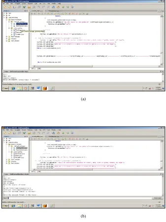
Tool is developed using NetBeans IDE. Outputs are shown in the form of (i) text, (ii) pictorial illustrations and (iii) table (database).

The text based view is shown in the output container (Figure 3).

The graphical view of the output is shown in the Frame [5], that contains the tasks (represented by task-id), COMPCost and COMMCost.

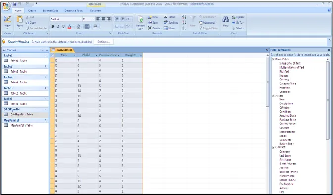
MS-Access is used to store the results in the form the task list.

4

. ALGORITHM

1. Algorithm eDAGitizer(n)

2. {

3. // n is the number of nodes that DAG can contain

4. HF=HeightFactor(n);// Calculate Height

Factor(levels)

5. MNPLT=n/HF;// Maximum Nodes Per Level by

Tool

6. read MNPLU;// // Maximum Nodes Per Level by

User

7. if(MNPLT=MNPLU)

8. {

9. Distribute nodes with respect to MNPLT

10. }

11. else

12. {

13. Revise Nodes per level and Height Factor

14. }

15. read choice of constructing DAG (1/0)

16. If (choice =1) then

17. DAG is generated with one node at entry and exit

level each

18. else

19. DAG is generated with any number of nodes (as per

MNPLT/MNPLU) irrespective of levels

20. for (i= 1 to (levels-1)) do // nodes at level having

maximum value will not have successors

21. {

22. for (j=1 to nodesat(i+1))

23. {

24. parent(i+1)(j)=random(node(i)(j))//choose

nodes(parents) from previous levels (predecessors), path(s) established

25. path=path+1;

26. } // for ‘j’ ends here

27. } // for ‘i’ ends here

28. for(i=1 to path)

29. Write tasklist; // task list will have path id, parent id,

child id

30. for(i=1 to path)

31. {

32. maintaining only one path between a particular

source and a particular destination //Eliminating multiple paths between the same source and destination

33. path1=path1+1; // number of paths may be reduced

after avoiding duplicates

34. }

35. for(i=1 to n)

36. {

37. weight(i)=random(MaxWeight);

38. compcost=compcost+weight(i);

39. }

40. for(j=1 to path1)

41. {

42. edgecost(j)=random(MaxCommunicationCost);

//edgecost(source,destination)

43. commcost=commcost+edgecost(j);

44. }

45. Compute CCR=Average(compcost) /

Average(commcost);

46. // displaying cost matrix

47. for(i=1 to n)

48. for(j=1 to n)

49. {

50. if(path(i,j)) //i-source, -destination

51. {

52. write edgecost;

53. } // ‘if’ ends here

54. } // ‘for’ ends here

55. for(all paths)

56. {

57. if(path(source, destination)

58. {

59. Find directpath(s);

60. Find indirectpath(s); // path with intermediate nodes

61. } //’if’ ends here

62. Leastcostpath(source,destination)=Min(Min(pathcos

t(alldirectpath)),Min(pathcost(all indirectpath));

63. }//’for’ ends here

64. }// Algorithm ends here

5. TIME COMPLEXITY

This tool has utilized Random Polynomial Time; An algorithm is said to be of polynomial time algorithm if its running time is upper bound by a polynomial expression in the size of the input for the algorithm, and the time

complexity is found to be, T(n) = O(nk) for some constant k,

where T(n) is the time to run the algorithm with n inputs,

O(nk_{) is the order of upper bound on the value of T(n)[15].}

6. IMPLEMENTATION AND RESULTS

The simulation results are shown below; Figure 2 shows the source code, Figure 3 shows the text description, Figure4

shows the graphic view in the Frame [16], and Figure 5 shows the stored table view.

(a)

(b)

5

(a) (b)

(c) (d)

Figure3. Sample output (text view)

(a) (b)

Figure 4. Frame with nodes, edges, COMPCost and COMMCost

Summary

Number of tasks =15

Number of edges=43

Total of all WEIGHTS =24

Total of all COMMUNICATION COSTS =101

Average Task Weight =1.0

Average Communication cost =2.0

CCR RATIO:2.0 Table of information related to start, end, cost of path, number of hops

______________________________________________________

path no.---start---end---cost of path---no. of hops

___________________________________________________

0---0---3---1---1

1---0---5---4---2

2---0---7---6---3

3---0---10---10---4

4---0---11---14---5

5---0---13---19---6

6---0---8---1---1

7---0---10---2---2

8---0---11---6---3

9---0---13---11---4

10---0---2---3---1

11---0---6---7---2

12---0---11---8---3

13---0---13---13---4

14---1---12---2---1

15---1---14---5---2

16---1---14---1---1

17---1---13---4---1

18---1---2---3---1

19---1---6---7---2

20---1---11---8---3

21---1---13---13---4

22---1---5---5---1

23---1---7---7---2

24---1---10---11---3

25---1---11---15---4

26---1---13---20---5

No of Paths =47 COST MATRIX ~~~~~~~~~~~~~~~~~~~~~~~~~~~~~~~~~~~~~~ 0 1 2 3 4 5 6 7 8 9

0 0 0 6 2 0 0 0 0 5 0

1 0 0 1 1 2 0 0 4 0 0

2 0 0 0 0 7 5 0 0 0 0

3 0 0 0 0 4 6 5 0 0 0

4 0 0 0 0 0 0 5 5 1 6

5 0 0 0 0 0 0 1 3 0 5

6 0 0 0 0 0 0 0 0 7 7

7 0 0 0 0 0 0 0 0 1 5

8 0 0 0 0 0 0 0 0 0 0

9 0 0 0 0 0 0 0 0 0 0

~~~~~~~~~~~~~~~~~~~~~~~~~~~~~~~~~~~~~~~ ~~~~~~

init:

deps-jar:

compile-single:

run-single:

GOD IS GREAT

Enter the number of tasks

:

10

Height Factor(approximated to)3

tasks per level(approximated to)3

Enter the maximum number of children:

3

DO YOU WANT ONE TASK TO BE at the starting level and end level then, press 1 to be yes otherwise press 0

1

Enter the number of Processors

2

Enter the Processing Speed of Processors

Processing Speed of Processor 0

5

Processing Speed of Processor 1

6

Enter the maximum Weight of the tasks:

5

Enter the maximum communication cost of the edges weight:

Figure 5. View of the table having the task list

7. CONCLUSION

DAGs are used to model data flow computation problems that involve indeterminism. Scheduling techniques are applied to optimize the resource utilization. Grid Computing is a technology that supports the arbitrary participation of resources and tasks. But resource mapping is still found to be very challenging. In this paper, the arbitrary participation of tasks is allowed to generate DAG and multiple lists of results have been observed by simulating with various different inputs. The tool shown in the paper is potentially developed to give expected results. The graphic view helps the uses to analyze the graph in a better way. The least cost path between the nodes improves the efficiency of scheduling in terms of communication cost. The cost matrix would be helpful to identify the path of no intermediate nodes and path of intermediate nodes. Also the least cost path between the source and destination nodes is found. The tool will be very much helpful to the researchers who are developing task scheduling algorithms for multiprocessor systems and for Grid computing environment.

8. ACKNOWLEDGEMENT

We would like to thank the almighty for being with us and making us to find the sparkling line in the midst of dark haze.

REFERENCES

[1] Maria M. Lopez, Elisa Heymann, Miquel A. Senar,”Analysis of Dynamic Heuristics for Workflow Scheduling on Grid Systems”, IEEE Proceedings of The Fifth International Symposium on Parallel and Distributed Computing,2006.

[2] Dr. D. I. George Amalarethinam, P. Muthulakshmi, “DAGITIZER – A Tool to Generate Directed Acyclic Graph through Randomizer to Model Scheduling in Grid Computing”, Proceedings f the second International Conference on Computer Science, Engineering and Applications, Vol. 2, Publisher: Springer-Verlag, pp. 969-978, 2012.

[3] Christofides, Nicos , Graph theory: an algorithmic approach, Academic Press, pp. 170–174, 1975.

[4] Thulasiraman, K.; Swamy, M. N. S., "Acyclic Directed Graphs", Graphs: Theory and Algorithms, John Wiley and Son, ISBN 9780471513568, 1992.

[5] Bang-Jensen, Jørgen, "2.1 Acyclic Digraphs", Digraphs:

Theory, Algorithms and Applications, Springer

Monographs in Mathematics (2nd ed.), Springer-Verlag, pp. 32–34, 2008.

[6] E. Ilavarasan, P. Thambidurai, R. Mahilmannan, “Performance Effective Task Scheduling Algorithm For Heterogeneous Computing System”, Proceedings of the Fourth International Symposium on Parallel and Distributed Computing, France, pp. 28–38, 2005.

[7] G.C. Sih, E.A. Lee,” A Compile-Time Scheduling

Heuristic For Interconnection-Constrained

Heterogeneous Processor Architectures,” IEEE Trans. Parallel Distributed Systems, Vol. 4 (2), pp. 175–187, 1993.

[8] J. Kim, J. Rho, J.-O. Lee, M.-C.Ko, CPOC: “Effective Static Task Scheduling For Grid Computing,” Proceedings of the 2005 International Conference on High Performance Computing and Communications, Italy, pp. 477–486, 2005.

[9] Yang, T and Gerasoulis, A, “PYROSS: Static Task Scheduling and Code Generation for Message Passing Multiprocessors”, Proceedings of 1992 International Conference on Super Computing (ICS ’92) Washington DC, July 19-23, K. Kennedy and C. D. Polychronopoulos Eds. ACM press, New York, pp. 428-437, 1992.

[10] Shirazi, B, Kavi, K, Hurson, A. R and Biswas, P, “PARSA: A Parallel Program Scheduling and

Assessment Environment”, Proceedings of the

International Conference on Parallel Processing, CRC Press Inc., Boca Raton, FL, pp. 68-72, 1993.

[11] Yu-Kwong Kwok, Ishfaq Ahmad, “Static Algorithms for Allocating Directed Task Graphs to Mutiporcessors,” ACM Computing Surveys, Volume 31, No., 4, December 1999.

[12] Chu, W. W., Lan, M. T., and Hellerstein, J, “Estimation

Applications in Distributed Processing Systems”, IEEE Transactions and Computing C-33, pp. 691-699, 1984.

[13] Hu, T. C. “Parallel Sequencing and Assembly Line Problems”, Operational Research 19, pp 841-848, 1961.

[14] Ellis Horowitz, Sartaj Sahni, Sanguthevar Rajasekaran, “Fundamentals of Computer Algorithms”, Galgotia Publications Pvt. Ltd., 2006.

[15] Sipser, Michael.” Introduction to the Theory of Computation”, Course Technology Inc. ISBN 0-619-21764-2, 2006.