The application of advanced computer models to the prediction of sound in enclosed spaces

(1)

THE APPLICATION OF ADVANCED COMPUTER MODELS

TO THE PREDICTION OF SOUND IN ENCLOSED SPACES

by

Mark John Howarth

This thesis was submitted for the degree of Doctor of Philosophy in the Department of Acoustics and Audio Engineering at the University of Salford.

(2)

-125-Glossary of symbols

Convolution

Absorption coefficient

6 Diffusion coefficient

6(s) Dirac delta function

Total energy at step N

Solid angle subtended from surface i to receiver

Oik Solid angle subtended from surface k to centre of surface i 0, Angle of incident sound ray from surface normal vector

0,. Angle of reflected sound ray from surface normal vector

Oim Angle subtended from element m on surface i to receiver (from surface normal)

A Diagonal matrix of surface reflection coefficients

A, Area of surface i

A ftft Area of element m on surface i dS Elemental area of a surface\

D(N) Vector of diffuse energy from ray tracing on all surfaces at t = N I

D," Diffuse energy from ray tracing on surface i at t = N I e" Vector of energy on all surfaces at t = N I

e," Energy on surface i at t = N I

E. Individual ray energy incident on surface i Eft Energy on surface i at time t

h(s) Linear system impulse response

Intensity incident on a surface

I(r) Reflected intensity at distance r from a reflecting surface Number of elements on surface

Number of surfaces in a model Markov-chain step number

(5)

Matrix of transition probabilities Distance from a reflecting surface

rim Distance from element m on surface i to receiver R(s) Cross-correlation of linear system input and output R.,„(s) Auto-correlation of linear system input

Time

Markov-chain time step length x(s) Linear system input

(6)

Abstract

Computer modelling of acoustics in enclosures has developed into various forms, none of which have yet demonstrated 100% accuracy. This thesis therefore details a study of room acoustic computer modelling. It highlights weaknesses with existing modelling techniques and describes the development and subsequent verification of an improved modelling technique.

The study discovers that for accurate prediction of many common room acoustic parameters diffuse reflections should be accounted for in the modelling of all reflection orders. However, many of the problems encountered in existing techniques are found to be caused by the way these diffuse reflections are modelled.

(7)

Chapter 1 Introduction

Since the first computer models of room acoustics of forty years ago', modelling techniques have evolved to a stage where they are currently used by some acousticians as a tool in the design of auditoria. Comouter models have an advantage over other design methods in that they are cost effective since they allow the designer considerable flexibility in the design process, where changes in materials or geometry can be tried and tested relatively quickly compared with, for instance, scale modelling techniques. Many modern programs also use their calculations as part of an `auralization' process to enable listeners to hear simulated room responses. However, despite the increasing complexity of computer models they are still not an 'indispensable tool' for the acoustician. One of the reasons for this is their questionable accuracy.

This was illustrated by a 1995 round-robin survey by Vorlandee, in which fourteen computer simulation programs were used to predict several acoustic parameters in a room. Program users were firstly given technical drawings detailing geometrical information along with qualitative descriptions of the materials within the room. Secondary tests were also carried out using identical absorption coefficients in each of the models. The predictions were then compared to measured values from the enclosure

(8)

-in the 1 kHz octave band. The study concluded that only three of the fourteen computer models produced 'unquestionably reliable predictions'. These three models, however, still produced errors greater than difference limens in at least 50 % of predictions.

To exploit fully the potential advantages of computer modelling in the design of enclosures, the accuracy of predictions therefore needs to be improved. This study addresses this need.

The key objectives of this study are therefore to

• highlight weaknesses with current modelling techniques • to develop an improved modelling technique.

The investigation methodology is as follows

a. A literature survey provides information on current computer modelling techniques used and their associated advantages and possible weaknesses b. Common room acoustic parameters specified in ISO 3382 3 are measured in eight

real enclosures

c. Predictions of these acoustic parameters in the eight enclosures are made using a computer model, identified in Vorlander's survey as reliable, and are compared with values measured in actual enclosures

d. Reasons for weaknesses in these predictions are hypothesized and areas for refinement are suggested

(9)

Chapter 2 Background

2.1 Geometrical room acoustics

Geometrical modelling of sound propagation is governed by Fermat's principle', which states that every wave propagates from the source to the receiver by way of the fastest path. In the case of room acoustics, sound propagates through air that can be considered as an isotropic, homogeneous medium at rest and the speed of sound can be regarded as constant. This means that sound propagates from the source to the receiver by way of the shortest path; that is, in a straight line or `ray'5.

Geometrical modelling therefore gives us the concept of sound rays, where energy from a sound source is divided into energy packets that propagate in straight lines away from the source. This is directly analogous to the concept of light rays in optics but has important differences which are discussed below. The analogy with light rays is useful since it gives us a way of visualizing reflection, diffraction and refraction of sound rays.

Reflections occur in every enclosed space since at some point a ray will meet a surface where it will at least partially be reflected. Geometric modelling of a reflection assumes

(10)

-3-Figure 2.1 Specular reflection from a smooth surface

the surface is perfectly smooth and has dimensions far greater than the wavelength of the incident sound. In optics, where wavelengths of visible light range from 0.3 to 0.8 pm, this is always the case but in acoustics wavelengths of audible sound be as long as 17 m, which few surfaces will reflect specularly. Where geometric assumptions are

not satisfied, diffuse or partially diffuse reflections may occur; these are discussed in section 2.3. Fermat's principle tells us that a ray propagating from a source and reflecting from a surface to a receiver will travel by the quickest route or, since the speed of sound can be taken as constant, by the shortest path. The reflection point is therefore such that the angle of reflection is equal to the angle of incidence. This is referred to as specular reflection and is illustrated in figure 2.1, where sound from source 'S' is reflected from a surface and received at point 'W.

2.2 Room acoustic computer modelling

2.2.1 Image-source method

(11)

Figure 2.2 Construction of image source, S,

and the image sources emit sound directly through them to the receiver.

A computer implementation of the technique was written by Gibbs and Jones' to calculate sound pressure levels within enclosures and the method was used to calculate echograms' by Santon ll and predict

reverberation times by Allen and Berkley'''. In 1982, Borish further refined the technique to allow the method to be used for more complex enclosures but noted that the number of image sources required increased exponentially with the desired length of decay'. The complexity of models was consequently limited by computation time. Lee and Lee" attempted to reduce calculation times by using a coordinate transformation method to eliminate non-visible image sources and therefore reduce the number of image calculations required. Their method also made more efficient use of computer memory, which meant more complex models could be modelled on computers with restrictive memory limitations.

One of the key advantages of the image-source method is that all possible reflection paths are found between source and receiver, which leads to a high time resolution of reflections. While one of its disadvantages is the required long computation time when high-order image sources are desired. Kristiansen, Krokstadt and Follestad 15 therefore developed a method of extrapolating low-order reflections to calculate high-order reflections as a way of speeding up the calculation process.

2.2.2 Ray-tracing method

The term 'ray tracing' is used here to represent all energy-particle tracing methods, where energy-particles can be represented by rays, beams, cones or pyramids. The method was first programmed for the modelling of room acoustics in 1958 by Allred and Newhouse' and developed by Krokstadt, Strom and Sorsdal 16 in 1967. As with the

(12)

-5-image-source method, it is based on geometrical acoustics.

In the ray tracing method, energy-particles are emitted from a source and reflected around a modelled enclosure. At each reflection, energy is taken from the particle according to the value of the reflecting surface's absorption coefficient. Particles are then 'collected' at a receiver position where their strengths and arrival times give an approximation of an energy decay after a sound source is switched off.

Ray tracing is more commonly used for modelling room acoustics than the image-source method because it is easier to program'', particularly for more complicated enclosure shapes. Its computation time also increases proportionally with the number of reflections modelled'', whereas with the image-source method, the computation time increases exponentially with the number of reflections'', which means more complex enclosures and longer decay times can be more easily modelled.

A further advantage of the ray-tracing method is that it can take non-specular effects into account. Several authors have therefore modified the method to account for non-specular reflections, these are discussed in section 2.4.

(13)

2.2.3 Hybrid models

The term 'hybrid' is used to describe modelling techniques that use a combination of ray tracing and the image-source method. They achieve this by using a ray-tracing algorithm to 'find' image sources, which are then used, as with the conventional image-source method, to radiate directly to the receiver. The problem, in conventional ray tracing, of determining an optimum 'ray-detector' size can therefore avoided and the locations of image sources can be calculated with greater ease for more complicated enclosures than with the conventional image-source method.

A cone-tracing technique by Maercke and Martin 20.21 used this concept to model early order reflections but because of computer memory limitations, higher order reflections were calculated with a conventional beam tracing algorithm. Their method used cones traced from image sources to determine whether image sources were valid. This eliminated the need to use finite-sized detectors around receivers.

Vorlander" developed a technique to calculate complete energy decays by using rays rather than cones to determine image-source locations. This method used ray tracing to determine the visibilities of image-sources and therefore retained the concept of ray detectors around receivers. The errors caused by this were neglected for reductions in computation time.

(14)

R2,,"

2.3 The importance of diffuse reflections

A diffuse reflection is one where sound incident on a surface is reflected into a wider solid angle than that of a specular reflection and is therefore not directly accounted for in geometrical modelling of acoustics. This scattering is attributable to wave effects caused by surface roughness, geometry and diffraction.

Diffuse reflections have an important role to play in the acoustics of rooms as they can improve the uniformity of a reverberant field and reduce the risk of areas of poor acoustics within a room". They also create a softer soudd and reduce the risk of undesirable echoes by improving the smoothness of the reverberant decay. In a study of surface diffusion by Hodgson' it was noted that in rooms with only specularly reflecting surfaces sound decays were non-linear with slopes decreasing with time causing rates of sound decay to be less than that predicted by Eyring's theory, especially in disproportionate rooms. However, in rooms with more diffuse surfaces, sound decays were more linear. Fricke and Haan26.27 conducted surveys asking musicians and music critics about their preferences for over fifty concert halls and compared these with objective features of the halls. They found that the feature that correlated best with their preferences was the diffusion of interior surfaces. This signifies the importance of accounting for surface diffusion in the design of such enclosures.

Diffuse reflections occur from 'rough' surfaces where the dimensions of the roughness are comparable to the wavelength

(15)

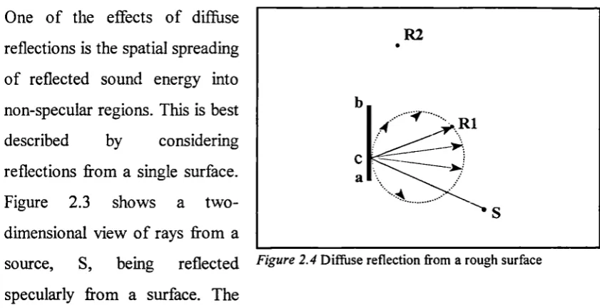
Figure 2.4 Diffuse reflection from a rough surface

[image:15.595.79.500.59.275.2]

One of the effects of diffuse reflections is the spatial spreading of reflected sound energy into non-specular regions. This is best described by considering reflections from a single surface. Figure 2.3 shows a two-dimensional view of rays from a source, S, being reflected specularly from a surface. The

region illuminated by these specular reflections is bounded by the paths given by reflections at points a and b. If the source and receivers shown are considered as points, and S radiates to all positions along the reflecting surface, it is clear that only one reflection, at position c, reaches Rl. Any receivers outside this illuminated zone, such as R2, receive no energy at all. If this specularly reflecting surface is now replaced by a diffusely reflecting surface, each incident ray, from S, is split by the surface into many weaker rays, reflecting out in a number of directions. Figure 2.4 shows a two-dimensional representation of a completely diffuse reflection from a rough surface. As in optics, this is described by Lambert's cosine law. Let us suppose a group of parallel rays with intensity I strike a surface along a small area dS at angle

q

from the surface normal, then the reflected intensity I(r) at angle or and distance r from the surface is given by

cos() cos(). I(r) = dS r

irr 2

If the incident angle is constant the received intensity is therefore proportional to the cosine of the reflection angle as represented by the circle in figure 2.4. The surface therefore reflects into all angles in 27c space so energy is received at R2. This spatial spreading of energy helps to make the reverberant field more diffuse.

In addition to spatial spreading, amplitude smoothing and temporal smearing makes the

(16)

-9-reverberant decay more linear. Energy reflected at position c by the diffusely reflecting surface is still received at R1 but with a lower amplitude than the specularly reflecting surface because incident energy at c is now dispersed in many directions. However, since energy is scattered at all positions along the reflector, energy is now also received at R1 from many other positions at slightly different times. This consequently smooths the reverberant decay at R1 in the time domain.

Diffusers also affect reflections in the frequency domain. With specularly reflecting surfaces reflections can produce a harsh sound equivalent to optical glare'. However, with 'fine-scale' diffusers, high frequencies are scattered and decays are smoothed, effectively reducing high-frequency energy from specular reflections. The diffusers therefore act like low-pass filters producing a mellower, softer tone. This is particularly noticeable where few diffusing surfaces are present but becomes less important when diffuse reflections are arriving from many directions'.

2.4 Computer modelling of diffuse reflections

In reality very few enclosures have only smooth surfaces that can be modelled specularly. Areas of seating and surfaces that are shaped or textured are common causes of diffuse reflections. It is therefore not surprising to find the need to include the modelling of diffuse reflections for accurate prediction of room acoustic parameters has been recognised by many authors'''. Vorlander noted that the three best programs in his survey all had algorithms that included the modelling of diffuse reflections. An overview of some techniques used to model such reflections is given here.

A 'diffusion coefficient' (sometimes referred to as 'diffusion factor'), 8, is often used to describe the fraction of reflected energy diffused by a surface and is therefore defined as the fraction of reflected energy directed non-specularly. If a is the absorption coefficient of a surface we can say:

(17)

where, incident energy = Ei absorbed energy = a E, diffused energy = 8(1 - a) E. specular energy = (1 - 8)(1 -

a)

E,

With ray-tracing methods, one method of modelling this energy reflected in non-specular directions would be to split rays into many weaker rays at each diffusely reflecting surface'. These new weaker rays would then each be traced and split further at each subsequent diffusely reflecting surface. However, this method has been rejected because the exponential increase in rays produced with time would result in long calculation times".

(18)

algorithm has to be repeated for each frequency band required, which further increases computation time.

Kuttruff and StraBen's re-direction method was developed further by Heinz' for auralization purposes. In this method specular reflections were calculated using a high-resolution hybrid method and a low high-resolution ray tracing was then performed using Kuttruff's method to create a diffuse decay. The specular and diffuse decays were then combined to give an overall energy decay. The calculations required were found to be time consuming so to reduce computation times only early reflection orders were modelled in this manner and the remaining 'reverberant tail' was modelled statistically so its 'gross temporal and spectral behaviour agrees with that of the true decay process'. Heinz indicated that this was only valid for rooms that are 'well-shaped' and that the method should not be considered for flat or long rooms.

In Naylor's method' the calculation procedure is divided into two sections. The first calculates early reflections according to geometrical acoustics theory using the conventional hybrid method. The second creates secondary diffuse sources at points where traced rays hit surfaces. These sources then radiate to visible receivers according to Lambert's cosine law (see section 2.3). The two sections are separated by a reflection transition order, so that diffusion is only modelled for reflection orders above this. Naylor developed this approach to predict 'long rich reflection sequences'n and considered that the 'pure' hybrid method could not produce these on a personal computer because a finite limit on the number of rays would have to be imposed, which would place an upper limit on the length of an accurate reflectogram obtainable.

(19)

Non-specular reflections were modelled by Gerlach' and Kruzins and Fricke' by using a radiant-exchange method based on Markov-chain theory. The method was not designed to specifically model diffuse reflections but to predict energy decays in semi-diffuse spaces. In this method energy is distributed from one surface to another at discrete intervals according to a transition probability. Each probability is calculated by dividing the visible solid angle projected onto a receiving surface by the total solid angle visible from the 'emitting' surface. This technique allows the shape of the room and the location of surfaces to influence the diffuse decay at a receiver. Gerlach compared predictions to scale model measurements where different combinations of absorptive and reflective surfaces were used. No diffuse surfaces were used in the model. Predicted results were found to correspond well except when only one wa il was absorptive. Kruzins and Fricke used their model to predict sound pressure levels in rooms containing internal barriers. They compared predictions with measurements in scale models and noted that their model did not account for edge diffraction effects and therefore limited comparisons to octave bands above 1 kHz. Predictions were found to correlate well with measured values.

A method that divided surfaces into interconnected nodes was developed by Kramer et al' in 1992. This method was similar to the radiant-exchange techniques described above but where surfaces were described by either specular nodes or diffuse nodes. For diffuse nodes energy was re-directed to another randomly-chosen node in a similar manner to Kuttniff's re-direction of rays. No validation of the program's predictions was presented by the authors so it is difficult to determine the accuracy of the technique.

Lewers' used a radiant-exchange method in combination with a specular ray-tracing method using triangular beams. Energy was subtracted at surfaces according to a diffusion coefficient and placed in a radiant-exchange procedure. The method was only used to predict reverberation times at a single frequency and computation times were not considered as the program was implemented on a fast mainframe computer. Comparisons were only made with reverberation time predictions using Sabine's formula in a single theoretical enclosure. It is therefore difficult to assess the accuracy of the

(20)

-13-technique.

In Borish's development of the image-source method' the filtering of specular reflections was proposed as a way of modelling diffuse reflections. This would involve convolution of measured or calculated responses of diffusors with incident sound. However, this approach would not model all aspects of diffuse reflections: the time-smearing effect of diffusion would be modelled but not the spatial scattering of energy. A similar method was proposed by D'Antonie. However, its accuracy cannot be assessed as the technique has not been implemented.

Lehnert and Blauertm illustrated how diffuse reflections would be regarded by the image-source method as 'image image-source clouds' surrounding conventional geometrical image sources. This was suggested by Dalenback, Kleiner and Svensson as a way of extending the image-source method to model diffuse reflections. However, they did not implement the method and claimed it would not be able to model all necessary reflection combinations.

(21)

discussed by the author and no validation against measured data was presented so it is difficult to assess the success of the technique.

2.5 Assessment of predictive accuracy

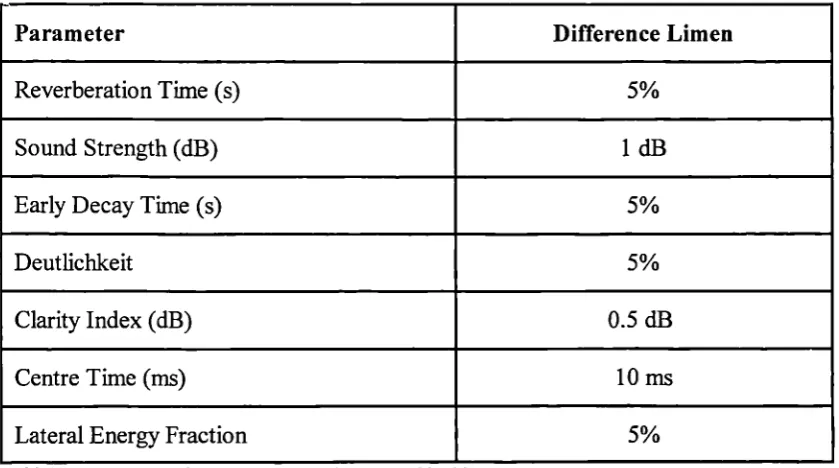
In order to assess the accuracy of models, errors in predicted acoustic parameters were compared to their subjective difference limens. A subjective difference limen (or threshold) is the change in a value that is just perceptible to a percentage of a population. The percentage normally used is 50 % so if errors are within difference limens, more than 50 % of a population would be unlikely to perceive a difference between the predicted value and the actual value, if heard.

Parameter Difference Limen

Reverberation Time (s) 5%

Sound Strength (dB) 1 dB

Early Decay Time (s) 5%

Deutlichkeit 5%

Clarity Index (dB) 0.5 dB

Centre Time (ms) 10 ms

[image:21.595.80.500.309.543.2]

Lateral Energy Fraction 5%

Table 2.1 Rounded subjective difference limens used in this study

The determination of subjective difference limens is complex because they are dependent upon the stimulus used. In 1958, Seraphim' determined that for reverberation times in the range 0.5 s to 2.0 s, a difference limen of approximately 4 % was appropriate. The study asked 500 tests subjects to compare decaying band-pass noise signals but determined the quoted difference limen by assessing the differences that 75 % of the subjects could perceive. Cremer and Miiller4 noted that for reverberation times below 0.6 s an absolute difference limen of approximately 0.024 s and that for reverberation

(22)

(23)

Chapter 3 Field Measurements

3.1 Description of enclosures

3.1.1 Overview of enclosures

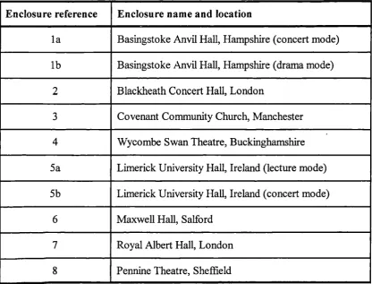
Eight enclosures were included in this investigation, two of which had variable acoustics and were studied in two different acoustic configurations. Table 3.1 shows the enclosures used along with their location and assigned reference number. The enclosures are specified by these reference numbers throughout the remainder of this text.

All the enclosures studied are commonly utilised for purposes where the acoustical behaviour of the space is of importance. This included five enclosures where orchestral concerts are performed; two theatres commonly used for drama and amplified music; two lecture theatres; a converted factory space, used for religious gatherings; and a general purpose University hall used for examinations, presentations and concerts. Two of the enclosures were designed as multi-purpose enclosures with variable acoustics. This enabled the prediction of acoustic changes to be assessed.

This varied mix of enclosure types represents the wide range of acoustic conditions

(24)

-17-commonly encountered and highlights some of the difficulties encountered in predicting the acoustic behaviour of such diverse conditions.

Enclosure reference Enclosure name and location

la Basingstoke Anvil Hall, Hampshire (concert mode) lb Basingstoke Anvil Hall, Hampshire (drama mode)

2 Blackheath Concert Hall, London

3 Covenant Community Church, Manchester 4 Wycombe Swan Theatre, Buckinghamshire 5a Limerick University Hall, Ireland (lecture mode) 5b Limerick University Hall, Ireland (concert mode)

[image:24.595.74.491.126.443.2]

6 Maxwell Hall, Salford 7 Royal Albert Hall, London 8 Pennine Theatre, Sheffield

Table 3.1 Enclosures used in investigation

3.2.1 Enclosure details

(25)

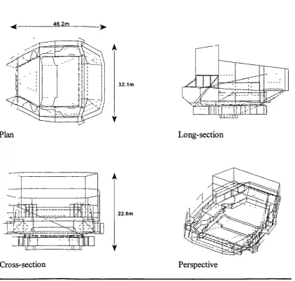
32.1m

22.6m

Enclosure 1

Plan Long-section

[image:25.595.74.497.155.557.2]

Cross-section Perspective

Figure 3.1 Views and overall dimensions of enclosure 1

Seated Capacity (approx) : 1400

Volume (approx) : 15000m3

Reverberation Time at 1 kHz : 1.8 s (drama mode), 1.9 s (concert mode)

Enclosure 1 is commonly used for drama, concerts and sporting events and changes configuration for each occasion. For this study configurations for drama and concerts were investigated. For concerts, absorption is largely provided by cloth-covered seating

(26)

-19-Figure 3.2 Source and receiver positions in enclosure 1

located on the main floor of the auditorium; in the choir area around the stage and along narrow side balconies. The seating in the front section of the main auditorium is bleacher seating that slopes to meet permanent seating at the rear of the enclosure. The side balconies contain four rows of seating. For the drama configuration, curtains are draped around the stage, which hide the choir seating from the auditorium. Similar curtains are draped along the side walls of the enclosure. Curved diffusers approximately 3 m high by 1.5 m wide are hung along the front of the side balconies for all configurations. Additional surface diffusion is provided by profiled wall shapes and the seating areas.

Responses were determined with a source (Si) located on the stage and six receivers located in the auditorium (R1 - R6). The positions of these are shown in figure 3.2. Coordinates of the positions used are presented in table 3.2.

Position x (m) _{Y (m)} z (m)

Si (stage) 9.60 -1.00 1.70

R1 (bleachers) 15.15 4.20 0.70

R2 (bleachers) 24.20 4.20 2.95

R3 (stalls) 35.10 5.00 6.95

R4 (stalls) 38.00 6.00 8.35

R5 (side balcony) 24.20 10.00 4.80

R6 (side balcony) 19.10 12.00 5.10

(27)

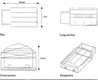
34.9m

A _J -4

'

17.6m

Long-section Plan

13.0m

[image:27.595.69.489.174.514.2]

Enclosure 2

Figure 3.3 Views and overall dimensions of enclosure 2 Seated Capacity (approx) : 600

Volume (approx) : 6800 m3

Reverberation Time at 1 kHz : 2.6 s

Enclosure 2 is commonly used for classical concerts. During the measurements, absorption was largely provided by heavy curtains covering the back stage wall and part of the rear wall of the main auditorium. During performances additional absorption is provided by the audience but only the unoccupied state was considered in this study. During measurements plastic seating, used during performances, was stacked at the rear

(28)

-21-Figure 3.4 Source and receiver positions in enclosure 2

of the hall leaving a clear wooden floor. The walls and barrel-vaulted ceiling were finished with lime plaster on laths. Surface diffusion was provided at high frequencies by ornamental plasterwork on the ceilings and around doorways.

Responses were determined with two sources (Si and S2) located on the stage and four receivers located in the auditorium (R1 - R4). The positions of these are shown approximately in figure 3.4. Coordinates of the positions used are presented in table 3.3.

Si (stage) -1.00 -1.00 1.70

S2 (stage) -6.40 3.75 1.70

R1 (auditorium) 5.50 -1.50 0.10

R2 (auditorium) 11.00 -6.83 0.10

R3 (auditorium) 14.50 -1.50 0.10

.

R4 (auditorium) 20.00 1 -4.00 0.10

(29)

30.0m

A

3.1m Enclosure 3

26.0m

Plan

Long-section

Cross-section

Perspective

Figure 3.5 Views and overall dimensions of enclosure 3

Reverberation Time at 1 kHz : 1.0 s

Enclosure 3 is commonly used for religious gatherings with music. It was converted from an existing factory space and therefore has a low ceiling height of 3.1 m and asymmetric geometry in the horizontal plane. Absorption is mainly provided from a carpeted floor covered by cloth-covered seats. Diffusion is mainly provided by the seats.

(30)

-23-• R2

• R5

• R7

• R6 • R4 -1

• R3

• R1

Figure 3.6 Source and receiver positions in enclosure 3

Responses were determined with a source (Si) located on a raised platform with seven receivers located in the auditorium (R1 - R7). The positions of these are shown in figure 3.6. Coordinates of the positions used are presented in table 3.4.

Si (floor) 4.40 0.00 2.03

R1 (seating) -0.70 -11.50 1.25

R2 (seating) 5.70 10.50 1.25

R3 (seating) 9.95 -10.30 1.25

R4 (seating) 11.40 11.20

— 1.25

-R5 (seating) 12.90 3.25 1.25

R6 (seating) 17.30 -9.00 1.25

R7 (seating) 19.10 -3.20 1.25

(31)

A

25.9m

, I I

-I

_MOSOMBETI

,

WINIIMEMilIMMINIR IMMINIMEMPINall

--\

MIZEMINIMMIHM-IM In

A

24.3m

Enclosure 4

34.6m

Plan Long--section

Figure 3.7 View and overall dimensions of enclosure 4

Enclosure 4 is commonly used for drama and amplified-music concerts. It has two rear balconies and absorption is mainly provided by cloth-covered seating, carpeted flooring and curtains draped around the stage. The area above the auditorium contains many acoustic reflectors, lighting rigs and walkways for technicians all of which act as diffusing elements along with the seating.

(32)

-25-Figure 3.8 Source and receiver positions in enclosure 4

Responses were determined with a source (Si) located on the stage and nine receivers located in the auditorium (R1 - R9). The positions of these are shown in figure 3.8. Coordinates of the positions used are shown in table 3.5.

Position x (m) Y (m) z (m)

S1 (stage) 9.50 3.50 1.40

R1 (stalls) 19.40 -1.20 0.25

R2 (stalls) 18.20 -8.20 2.00

R3 (stalls) 26.80 -1.25 4.30

R4 (2nd balcony) 29.00 -2.35 9.50

R5 (2" balconY) 32.50 -4.50 12.00

R6 (2"d balconY) 31.50 -7.00 12.00

R7 (stalls) 25.90 -4.90 1.00

R8 (1 5' balcony) 31.00 -3.10 6.20

(33)

32.0m

1Nu

mi il

ill

il

III

11111111KIIII

d1

2111r

Mini

I

\ r

A

14.6m

Perspective Enclosure 5

41.0m

Plan Long-section

[image:33.595.76.525.154.541.2]

Cross-section

Figure 3.9 Views and overall dimensions of enclosure 5 Seated Capacity (approx) : 1000

Volume (approx) : 9400 in3

Reverberation Time at 1 kHz : 1.2 s (lecture mode)to 1.4 s (concert mode)

Enclosure 5 is commonly used for lectures and concerts and changes configuration accordingly. In this study both configurations were investigated. For concerts, absorption is largely provided by cloth-covered seating located in the main auditorium, in the choir area behind the stage and in the side balconies. For the lecture configuration curtains are draped around the stage, including between the choir seating and stage, and

(34)

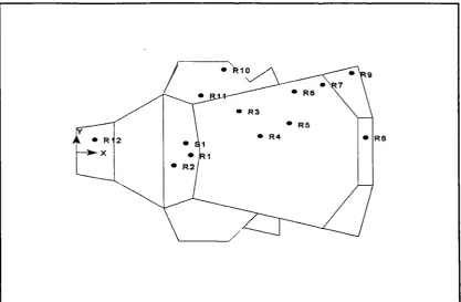
-27-Figure 3.10 Source and receiver positions in enclosure 5

absorbent banners extend across the main auditorium. The walls are of unfinished blockwork providing high-frequency diffusion and reflectors are suspended above the stage and auditorium to diffuse low frequencies while reflecting high frequencies.

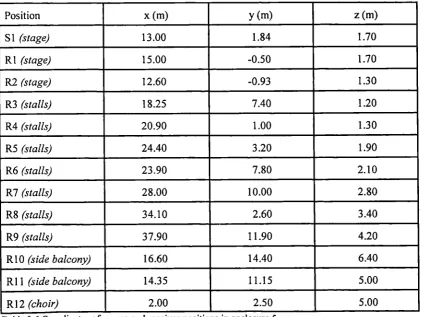
[image:34.595.78.496.66.339.2]

(35)

Si (stage) 13.00 1.84 1.70

R I (stage) 15.00 -0.50 1.70

R2 (stage) 12.60 -0.93 1.30

R3 (stalls) 18.25 7.40 1.20

R4 (stalls) 20.90 1.00 1.30

R5 (stalls) 24.40 3.20 1.90

R6 (stalls) 23.90 7.80 2.10

R7 (stalls) 28.00 10.00 2.80

R8 (stalls) 34.10 2.60 3.40

R9 (stalls) 37.90

_

11.90 4.20

RIO (side balcony) 16.60 14.40 6.40

R11 (side balcony) 14.35 11.15 5.00

[image:35.595.81.503.64.381.2]

R12 (choir) 2.00 2.50 5.00

(36)

20.8m

11.1m

Cross-section Perspective

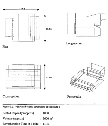
Enclosure 6

33.6m

A

Long-section

Plan

Figure 3.11 Views and overall dimensions of enclosure 6

Seated Capacity (approx) : 1000 Volume (approx) : 5600 m3

[image:36.595.67.498.111.614.2]

(37)

• R9 • R7

• I

R54, R8

•

mi

I(

T),.. x

•

s1

• R2 • R1

1

[image:37.595.77.498.62.268.2]

• R3

present. The rear wall of the stalls, located under the balcony is formed by sliding wooden doors that separate a storage room from the main auditorium. The walls and ceiling are finished with smooth painted plasterwork and no diffusers are present. The seating areas are therefore the main diffusing surfaces in the enclosure.

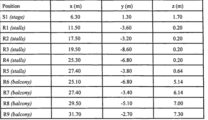
Responses were determined with a source (Si) located on the stage and nine receivers located in the auditorium (R1 - R9). The positions of these are shown in figure 3.12. Coordinates of positions used are presented in table 3.7.

SI (stage) 6.30 1.30 1.70

R1 (stalls) 11.50 -3.60 0.20

R2 (stalls) 17.50 -3.20 0.20

R3 (stalls) 19.50 -8.60 0.20

R4 (stalls) 25.30 -6.80 0.20

R5 (stalls) 27.40 -3.80 0.64

R6 (balcony) 25.10 -6.80 5.14

R7 (balcony) 27.40 -3.40 6.14

R8 (balcony) 29.50 -5.10 7.00

R9 (balcony) 31.70 -2.70 7.30

Table 3.7 Coordinates of source and receiver positions used in enclosure 6

[image:37.595.80.508.476.722.2]

(38)

-31-72.6m

Plan

A Enclosure 7

I I I • maa

70.0m

1111"

limmumwrimm

4WilIMINMINNINgINNEMIN

-`AIMINIMIVAIPY

Long-section

81.0m

Volume (approx) : 11O,000 m3

Reverberation Time at 1 kHz : 2.9 s

[image:38.595.76.507.167.643.2]

(39)

[image:39.595.79.502.77.376.2]

behind the stalls seating and above this is a "First Tier" of private boxes, a "Second Tier" of open boxes and a balcony. Choir seating is also situated behind the stage. In its unoccupied state, absorption is mainly provided by the cloth-covered seats and heavy curtains draped around private boxes.

Diffusion is provided from ornamental plasterwork on the balcony and box fronts and from curved "mushroom" diffusers suspended from the dome ceiling, which occupy approximately 50% of the plan area. Mineral fibre is attached to the top of the diffusers to reduce the strength of reflections from the dome ceiling, which had previously caused flutter echoes'. Large organ pipes located behind the stage also provided a diffuse surface.

Responses were determined with a source (Si) located on the stage and twelve receivers located in the auditorium (R1 - R12). The positions of these are shown in figure 3.14. Coordinates of the positions used are presented in table 3.8.

(40)

-33-Position x (m) _{Y (m)} z (m)

Si (stage) 0.00 -14.50 2.50

R1 (stage) 4.70 -14.50 2.05

R2 (choir) 8.00 -20.00 3.00

R3 (arena) 4.50

_

-6.00 1.70

R4 (stalls) 3.00 14.50 2.50

R5 (stalls) 14.00 10.00 3.50

R6 (grand tier) 21.00 -3.00 7.45

(choir)

• R7 -10.50 -20.00 6.00

R8 (second tier) -17.00 13.50 11.05

R9 (second tier) -20.00 -6.00 11.05

,

(balcony)

. R10 22.00 -15.00 17.50

R11 (balcony) , 21.00 15.00 17.00

[image:40.595.79.497.64.394.2]

R12 (balcony) -5.00 30.00 19.00

(41)

< 23.0m >-A

19.5m

I'

A

8.0m

Enclosure 8

Plan _Long-section

Cross-section _Perspective

Enclosure 8 is commonly used for lectures and classical concerts. It is asymmetric in plan with a concave side wall. When unoccupied absorption is mainly provided by cloth-covered seats, curtains draped over the front wall (behind the 'stage' area) and by acoustic treatment on the rear wall.

[image:41.595.81.498.165.561.2]

(42)

-35-Figure 3.16 Source and receiver positions in enclosure 8

Reflective panels that cover 80% of the plan above the seating are suspended from the ceiling.

Responses were determined from a source (Si) located on the 'stage' (this was an area of flooring at the front of the enclosure that was not raised) and from a source (S2) located to the rear of the seated area. Five receiver positions (R1 - R5) were used throughout the auditorium. The positions used are shown in figure 3.16 with their coordinates presented in table 3.9.

Si (floor) 3.20 4.50 1.70

S2 (seating) 21.20 7.85 6.70

R1 (floor) 7.70 3.80 2.00

R2 (seating) 11.90 -1.50 3.60

R3 (seating) 13.80 6.00 4.20

R4 (seating) 17.50 -0.10 5.40

[image:42.595.73.496.60.316.2]

R5 (seating) 20.00 -7.40 6.70

(43)

3.2 Measurement procedure

3.2.1 Instrumentation

The following equipment was used during the measurements

Description Make Type Serial Number

Portable Computer Compaq Portable II 1806BE4F0060 Data acquisition card DRA Labs AD2-160 582

Microphone B & K 4165 1547261

Microphone B & K 4165 1547260

Microphone AKG C414 EB/48 25117

Microphone pre-amplifier B & K 2639 1527966 Microphone pre-amplifier B & K 2639 1527964

Microphone pre-amplifier Salford U. - SUO2

Measurement amplifier B & K 2610 1501539

Power amplifier Quad 306

-Dodecahedron sound source Salford U. - SUO1

Temp. and humidity meter Comark 2020 108614

Calibrator B & K 4230 431601

(44)

[image:44.595.84.503.31.705.2]

(45)

3.2.2 Measurement setup

The measurement chain was set up as shown in figure 3.17. Measurements of acoustic impulse responses were made at fixed positions in the enclosures in order to determine room acoustic parameters. Source and receiver positions were chosen to represent those normally encountered in each enclosure. For example, in an auditorium the source would be placed on the stage and various receiver positions would be chosen throughout the audience area. In certain halls receiver positions were also chosen to investigate specific acoustic features. Receivers under balcony overhangs were chosen to lock at the prediction of acoustic shadowing, while positions close to diffuse surfaces were used to examine the modelling of surface diffusion. In certain enclosures flutter echoes could be heard. Consequently, source-receiver positions were chosen to investigate this feature. During measurements the source centre was located at a height of 1.7 m above the floor corresponding to the average mouth height of a standing speaker. Receiver microphones were positioned at a height of 1.2 m above the floor to correspond to ear height of average listeners in typical chairs.

(46)

Omni-directional microphone measurements were performed at all receiver positions chosen. Measurements using the figure-of-eight microphone were only made at selected positions because of time constraints. The figure-of-eight microphone was orientated so it 'faced' the source at each receiver position. That is, with its figure-of-eight axis perpendicular to the source-receiver line, as shown in figure 3.18. To minimise measurement uncertainty sixteen impulse responses were averaged at each receiver position.

For the omni-directional microphone measurements, the system was calibrated before each set of measurements using a 1000 Hz tone at 93.8 dB. After each set of measurements the calibration level was again checked. A calibrator was not available for use with the AKG C414 figure-of-eight microphone. However, impulses derived from the figure-of-eight measurements were only used for calculating early lateral energy fractions. Since the AKG C414 microphone has switchable directivity, it was also used for additional omni-directional measurements. Any calibration errors were then cancelled out during the calculation of the parameter (see Appendix A). To reduce any errors due to drift all instrumentation used was allowed a `warm-up time' of approximately ten minutes. Figure-of-eight and omni-directional measurements using the AKG C414 were made alternately at each receiver position.

Temperature and relative humidity were recorded at the start and end of each set of measurements to determine the speed

of sound and for the calculation air absorption in the predictive models.

The software and data acquisition card used employed a maximum-length sequence (MLS) system (see

(47)

3.2.3 The maximum-length sequence measurement method

The MLS method is a way of determining the impulse response of a linear system by cross-correlating a pseudo-random input noise with the measured output of the system. In room acoustics the transfer of sound between a source and receiver in an enclosure can be regarded as a linear system provided there are no significant variations in the characteristics of the system over the measurement period. Use of the method in room acoustics was pioneered by Schroeder" in the 1960's because it has important advantages over conventional impulse test methods for the measurement of sound decay. A problem encountered with impulse test methods is the requirement of the sound source to provide a powerful acoustic impulse over a wide frequency range. Traditionally, pistol shots and balloon bursts were used because they provided a powerful acoustic response although the spectra produced were not flat'. Impulses input into loudspeakers produced flat spectra but often could not radiate sufficient power to produce required signal-to-noise ratios in concert halls. Pseudo-random noise has a flat spectrum and for the same energy as a single impulse has a peak amplitude that is typically 100 times smaller'. This means it can be used to drive a loudspeaker to achieve considerable improvements in the signal-to-noise ratio of measured impulse responses'. Since the method cross-correlates the measured output with a known input it is also an effective way of reducing the influence of extraneous noise during measurements'. Since the input signal is deterministic and repeatable, impulse responses can be averaged to improve the signal to noise ratio. Any unwanted uncorrelated noise will then be averaged over the number of repeated sequences. The signal to noise ratio improves by 3 dB for every doubling of the number of sequences". In comparisons of different methods for measuring reverberation times by Vorldnder and Biete techniques utilising broad-band pseudo-random sequences, such as MLS, were considered the most powerful available.

From signal theory' we know that, for a linear system, the cross-correlation between the input x(s) and the output y(s) is equal to the convolution of the system's impulse response with the auto-correlation of the input.

i.e. R„y(s) = R„„(s) * h(s)

(48)

-41-The result of convolving a sequence with a pure impulse, represented by a dirac delta function (5(s), is the sequence itself Therefore, if the auto-correlation of the input signal is a dirac delta function, the cross-correlation of the input x(s) and the output y(s) is equal to the impulse response h(s).

i.e. _R(s)= 8(s) * h(s) = h(s).

3.2.4 Calculation of acoustic parameters

(49)

Chapter 4 The Conventional Hybrid Model

4.1 Description of the computer model

Models of enclosures were created using ODEON v.2.5 61 developed at the Technical University of Denmark. In order to assess the performance of existing modelling techniques it would be preferable to compare predictions from a wide variety of algorithms but due to financial constraints this was not possible. However, ODEON was one of the three most accurate programs tested in Vorlander's round-robin survey' and can therefore be considered as representative of the best of contemporary modelling techniques.

The model used a modified form of the hybrid ray tracing / image source method, where the calculation is split into two parts by a reflection 'transition order'. Reflections occurring before the transition order are referred to as 'early' reflections and were modelled using specular image sources. Those following it are called 'late' or 'reverberant' reflections and were modelled by secondary diffuse sources located at reflection points.

(50)

-43-The image sources used for the modelling of early reflections were generated using a conventional hybrid method. All reflection orders up to and including the transition order were therefore modelled specularly. For the calculation of latz reflections ray tracing continued but secondary diffuse sources instead of specular image sources were created at each subsequent surface reflection. These secondary sources were elemental area sources that radiated diffusely into the room from the point of reflection. After the generation of a secondary source the energy was re-grouped back into the primary ray that created it. This ray was then traced forward with a direction determined by Kuttruff's re-direction method. That is, a random number between zero and one was generated, if it was greater than the surface's diffusion coefficient the ray was reflected in a purely specular direction. Otherwise a reflection direction was randomly chosen from a distribution following Lambert's law.

4.2 Accuracy of input data

In any assessment of predictive models the accuracy of the model's input data is of importance. The input data required for the computer models here divides into the following areas

• geometry

• absorption coefficients • diffusion coefficients.

4.2.1 Geometry of enclosures

Table 4.1 shows sources of geometrical data for each of the enclosures. For enclosures where fill architectural drawings were available, detailed plan and sectional views gave accurate geometrical input data for the models.

(51)

ceiling height is a recognised source of error but was not considered to unduly influence the predictions because the source positions used were located on the stage, which had its own low ceiling. Reflected sound energy from the vaulted ceiling was therefore not prominent in the measured responses because it mainly consisted of reflections greater than the second order that arrived relatively late, that is, mostly after 80 ms. Enclosure 6 had a large balcony at the rear of the hall that contained raked seating. It was therefore possible to measure the height of the balcony and reach the ceiling from the rear of the balcony to determine its height. The main estimated dimension in enclosure 6 was the height of the fly-tower. By viewing the external dimensions of the hall it was possible to see that the fly-tower was only slightly higher than the auditorium ceiling so this was used in the model. However, any errors in the estimated height of the fly-tower were not considered significant because it was lined with sound absorbent material and contained absorbent stage curtains, which reduced the influence of reflections from it.

Enclosure Source of geometrical data 1 Full architectural drawings

/ _{Architectural plan, measurements and estimation}

3 Measurements

4 Full architectural drawings 5 Full architectural drawings

6 Architectural plan, measurements and estimation _

[image:51.595.90.527.364.585.2]

7 Full architectural drawings 8 Full architectural drawings Table 4.1 Sources of geometrical data

No architectural drawings were available for enclosure 3 but the geometry was relatively simple and the dimensions were small and easily measured.

The geometries of enclosures was input into the computer program by creating plane surfaces using corner points: corner points were entered as 3-dimensional coordinates

(52)

-45-and then linked together to form plane surfaces.

4.2.2 Absorption coefficients of surfaces

For enclosures 1, 4 and 5 measured absorption coefficients for seating areas were supplied by acoustic consultancies involved in the original design 63,64. However, for other enclosures and surfaces measured absorption coefficients were not available. Values used were therefore mainly selected from an absorption coefficient library provided with the program or from literature65,66,67,68 . This is a recognised source of potential inaccuracies but it is impossible to determine errors in values used without direct measurement of the absorption coefficients of actual materials, which was not possible due to financial constraints. However, since each enclosure contains several different surface treatments and enclosures differ from each other, negative and positive errors in coefficients used should average out when all enclosures are considered. Any analysis of predictive errors encountered in individual enclosures should account for absorption coefficient inaccuracies as a potential cause of problems.

4.2.3 Diffusion coefficients of surfaces

A standard method for measuring diffusion coefficients of surfaces does not currently exist. However, a current research programme° led by Dr T J Cox at the University of Salford is investigating this problem. For the purposes of this study model surfaces were therefore classified as either 'rough' or 'smooth'. This simplification has been used with some success in previous studies comparing predictions with scale model measurements'. A surface representing audience seating was considered highly diffusing or 'rough' and was assigned a high diffusion coefficient. A painted plaster surface or similar was considered 'smooth'.

(53)

diffusion coefficients were used in the calculation of all reflection orders. For simplification, only 'smooth' surface diffusion coefficients were varied because in most of the enclosures studied the majority of surfaces were considered 'smooth'.

Research by Lam." indicated that diffusion coefficients of 0.1 and 0.7 were best suited for smooth and rough surfaces respectively and noted that a diffusion coefficient of 0.0 was not suitable for accurate predictions. These results were used as guide for the coefficients used in this study. A diffusion coefficient of 0.7 was therefore used for rough surfaces such as areas of seating. To study the influence of changes in diffusion coefficients those on smooth surfaces were varied between values of 0.05, 0.1, 0.2 and 0.4. Smooth rather than rough surface coefficients were varied because the majority of surfaces were considered smooth and many of the rough surfaces were highly absorptive so a stronger more discernible effect on predictions was expected.

4.3 Modelling of early reflections

The importance of early reflections on the subjective impression of listeners has been noted by many acousticians' and has engendered the development of various objective acoustic parameters73.74'75. It was therefore considered important to investigate the effect of modelling early reflections using different techniques. This was possible with the program used because it had the capability to model early reflections using a specular method or by using diffuse secondary sources. This choice was determined by the program's transition order parameter. Therefore, predictions in each enclosure were made with transition order values of zero, one, three and five, with diffusion coefficients held at 0.1 and 0.7. With a transition order of zero, all reflections were modelled diffusely; with a transition order of five, the first five reflections were modelled specularly.

Table 4.2 summarises the combination of diffusion coefficients and transition orders employed for each enclosure model.

(54)

-47-Ds, Dr TO 0 TO 1 TO 3 TO 5

0.05, 0.7 V - -

-0.1, 0.7 i i V i

0.2, 0.7 i - -

-0.4, 0.7 .1 - -

(55)

Chapter 5 Performance of the Hybrid Model

5.1 Assessment of model performance

The performance of the hybrid model was assessed by comparing its predictions of room acoustic parameters with measured values. These comparisons were analysed in two stages both of which are presented in this chapter.

In the first stage, presented in section 5.2, an overall indication of accuracy is given by comparing errors averaged over all receiver positions measured. For most of the parameters, this is eighty-five receiver positions over ten enclosures (including different enclosure configurations). For lateral energy fraction a separate measurement set-up was required so only forty-four receiver positions were compared. This overall view of comparisons gives an indication of the performance of the model for the prediction of various parameters at different frequencies and illustrates how changes in the way reflections are modelled influence average predictive accuracy.

However, the overall performance of the model does not illustrate what happens in individual enclosures. Therefore to understand the model's behaviour in detail, its

(56)

-49-performance for each enclosure was examined at individual receiver positions. This second analysis stage is presented in section 5.3.

5.2 Overall prediction of room acoustic parameters

5.2.1 Prediction of reverberation time

The effect of transition order variation on the prediction of reverberation time is shown in table 5.1. Values shown are averaged over all receiver positions in all enclosures.

Frequency

(Hz)

TO 0 TO 1 TO 3 TO 5

Mean Error (%) Standard Deviation in Error (%) Mean Error (%) Standard Deviation in Error (%) Mean Error (%) Standard Deviation in Error (%) Mean Error (%) Standard Deviation in Error (%)

125 31.0 48.5 31.3 47.7 30.8 47.8 36.5 48.0

250 28.0 55.7 27.3 54.8 27.9 55.1 31.9 55.1

500 _

9.2 32.2 10.7 31.8 12.4 31.1 16.1 34.3

1000 0.6 25.4 2.9 25.7 5.9 24.9 9.0 26.8

2000 -0.9 22.2 1.2 22.2 4.3 22.5 7.0 23.6

4000 -0.4 20.5 1.7 _ 21.1 3.8 22.3 8.1_ 22.2

Table 5.1 Effect of varying transition order on prediction of reverberation time (Ds = 0.1, Dr = 0.7)

At low frequencies transition orders of zero, one and three produced similar average errors while at higher frequencies variation in transition order had a greater influence on results. Overall, a transition order of zero produced the smallest average errors. This is clearer at mid- to high frequencies while at lower frequencies transition orders of one and three resulted in similarly low errors. All transition orders produced similar standard deviations in errors. This indicates that, for the most reliable predictions of reverberation time, diffuse effects should be included for all reflections and not introduced at higher reflection orders.

(57)

The effect of smooth surface diffusion coefficient (Ds) variation on the prediction of reverberation time is shown in table 5.2. Values shown are averaged over all receiver positions in all enclosures.

Frequency

(Hz)

Ds 0.05 Ds 0.1 Ds 0.2 Ds 0.4

Mean Error (%) Standard Deviation in Error (%) Mean Error (°/0) Standard Deviation in Error (%) Mean Error (%) Standard Deviation in Error (%) Mean Error (%) Standard Deviation in

Error (%)

125 63.7 109.3 31.0 48.5 34.5 48.8 25.2 47.7

250 72.4 142.3 28.0 55.7 30.9 57.9 23.8 56.4

500 56.8 170.3 9.2 32.2 13.0 44.4 5.9 34.5

1000 32.0 110.3 0.6 25.4 1.6 28.7 -3.0 26.5

2000 20.4 69.6 -0.9 22.2 -0.4 19.6 -3.7 21.6

4000 12.3 39.4 -0.4 20.5 0.6 17.4 -1.6 20.3

Table 5.2 Effect of varying diffusion coefficient on prediction of reverberation time (TO = 0, Dr = 0.7)

At low to mid-frequencies a diffusion coefficient of 0.4 on average produced the most reliable predictions with the smallest errors and the lowest standard deviations in errors. A diffusion coefficient of 0.05 resulted in high average errors and standard deviations. However, at higher frequencies lower diffusion coefficients of 0.1 and 0.2 produced the most reliable predictions. As with predictions shown with variation of transition order, only average errors at 1000 Hz and above were within a difference limen of 5%. However, a notable decrease in low frequency errors did occur when smooth surface diffusion coefficients were increased. This indicates that, for prediction of reverberation time, smooth surface diffusion coefficients should be defined in the frequency domain with higher values at low frequencies and lower values at high frequencies. One of the reasons for needing higher smooth surface diffusion ,z,oefficients at low frequencies is that the wavelengths of sound at these frequencies are comparable to many of the reflecting surface dimensions. This means scattering of sound occurs from surface edge diffraction and the assumptions of geometrical sound reflection become invalid. Factors affecting the prediction of room acoustic parameters at low frequencies are discussed further in subsection 5.3.1

At mid- to high frequencies a smooth surface diffusion coefficient of 0.1 or 0.2 produced the smallest average errors, which agrees with similar previous findings by Lam m'. A

(58)

-51-lower coefficient of 0.05 produced over-predictions while a higher diffusion coefficient of 0.4 produced under-predictions. A possible explanation for this is that as diffusion coefficients are increased the randomization of ray directions is increased. On average this results in more energy being more evenly distributed around an enclosure which means more energy is incident upon absorptive areas, such as seating. This causes a more rapid decay of energy in the modelled enclosure and consequently shorter reverberation time predictions. This agrees with research by Hodgson that concluded that in rooms with only specularly reflecting surfaces the rate of sound decay is less than that predicted by Eyring theory.

5.2.2 Prediction of sound strength

Frequency

(Hz)

TOO TO 1 TO 3 TO 5

Mean Error (dB) Standard Deviation in Error (dB) Mean Error (dB) Standard Deviation in Error (dB) Mean Error (dB) Standard Deviation in Error (dB) Mean Error (dB) Standard Deviation in Error (dB)

125 6.5 5.8 6.6 5.8 6.8 5.8 6.6 5.7

250 2.6 4.2 2.7 4.1 2.9 4.1 2.8 4.1

500 1.4 3.2 1.6 3.2 1.8 3.2 1 7 3.2

1000 0.6 2.7 0.8 2.7 1.1 2.6 1.0 2.6

2000 -0.0 2.4 0.2 2.4 0.4 2.3 0.4 2.3

4000 0.5 2.5 0.8 2.6 1.0 2.6 1.0 2.6

Table 5.3 Effect of varying transition order on prediction of sound strength (Ds = 0.1, Dr = 0.7)

Table 5.3 and table 5.4 show average errors in the prediction of sound strength with variation in transition order and diffusion coefficient respectively. Values shown are averaged over all receiver positions in all enclosures.

(59)

table 5.4.

Frequency

(Hz)

DS 0.05 Ds 0.1 Ds 0.2 Ds 0.4

-Mean Error (dB) Standard Deviation in Error (dB) Mean Error (dB) Standard Deviation in Error (dB) Mean Error (dB) Standard Deviation in Errur (dB) Mean Error (dB) Standard Deviation in Error (dB)

125 6.4 5.9 6.5 5.8 6.4 5.9 6.3 5.9

250 2.6 4.2 2.6 4.2 2.5 4.2 2.4 4.3

500 1.4 3.2 1.4 3.2 1.4 3.2 1.2 3.3

1000 0.6 2.7 0.6 2.7 0.6 2.7 0.4 2.8

2000 -0.1 2.4 -0.0 2.4 0.0 2.4 -0.2 2.5

4000 0.5 2.6 0.5 2.5 0.6 2.6 0.4 2.7

Table 5.4 Effect of varying diffusion coefficient on prediction of sound strength (TO = 0, Dr = 0.7)

5.2.3 Prediction of early decay time

The effect of transition order variation on the prediction of early decay time is shown in table 5.5. Values shown are averaged over all receiver positions in all enclosures.

As early decay time is calculated in a similar manner to reverberation time it is useful to compare the resulting errors from their respective predictions. Reverberation time is determined from the slope of the decay between the -5 dB point and the -35 dB point; early decay time is determined from the slope of the decay from the 0 dB point to the -10 dB point. The accuracy of early decay time predictions is therefore affected more by the modelling of early reflections. This is apparent from the values shown in table 5.5, which vary more with transition order than equivalent values for reverberation time (see table 5.1).

Frequency

(Hz)

TO 0 TO 1 TO 3 TO 5

Mean Error (%) Standard Deviation in Error (%) Mean Error (%) Standard Deviation in Error (%) Mean Error (%) Standard Deviation in Error (%) Mean Error (°/0) Standard Deviation in

Error (%)

125 26.9 60.8 23.3 60.5 20.1 56.5 24.7 59.4

250 21.1 60.7 17.1 60.0 15.2 58.9 15.9 60.6

500 -1.1 40.0 -3.0 39.2, -5.2 39.1 -5.5 46.4

1000 -3.5 34.1 -4.4 36.0 -9.2 33.6 -9.6 41.4

2000 -5.2 31.1 -6.6 33.6 -12.4 27.4 -15.0 30.6

4000 -4.6 31.2 -6.1 34.0 -14.1 27.1 -18.1 28.8

Table 5.5 Effect of varying transition order on prediction of early decay time (Ds = 0.1, Dr = 0.7)

(60)

-53-The standard deviations in errors for early decay time predictions were also notably higher than for reverberation time predictions. This is possibly because any variations in determination of the slope of the 10 dB decay are multiplied by six to calculate early decay time, whereas for reverberation time the slope is determined over a 30 dB range and any variations are only doubled.

As with reverberation time, the smallest average errors at mid- to high frequencies occurred with a transition order of zero indicating that the modelling of diffusion should be included in all reflection orders. At low frequencies a transition order of three produced the smallest errors. This is probably because the introduction of specular reflections decreases the gradient of the energy decay, which at low frequencies is steeper than it should be due to other factors (see subsection 5.3.1). If these other factors were removed, the predicted decay at low frequencies would possibly also require the introduction of diffuse modelling from the first order reflection.

At low frequencies average errors in the prediction of early decay time were smaller in magnitude than for reverberation time. Average errors at mid- to high frequencies were generally larger in magnitude and were all negative, showing under-predictions. This differs from reverberation time, where average errors mainly showed over-predictions. This indicates possible problems with the prediction of early energy and suggests that the early part of the modelled energy decay slope is too steep. The modelling of this early energy is investigated in more detail in subsection 5.3.2.

The effect of changing the diffusion coefficient of smooth surfaces (Ds) on the prediction of early decay time is shown in table 5.6. Values shown are averaged over all receiver positions in all enclosures.

(61)

Frequency

(Hz)

Ds 0.05 Ds 0.1 Ds 0.2 Ds 0.4

Mean Error (%) Standard Deviation in Error (%) Mean Error (%) Standard Deviation in Error (%) Mean Error (%) Standard Deviation in Error (%) Mean Error (%) Standard Deviation in Error (%)

125 34.6 61.4 26.9 60.8 26.5 56.9 23.6 57.6

250 37.0 79.2 21.1 60.7 21.8 58.3 19.8 58.2

500 17.2 87.2 -1.1 40.0 1.0 41.4 -0.4 38.0

1000 11.7 71.1 -3.5 34.1 -1.5 35.0 -2.1 31.9

2000 0.4 35.9 -5.2 31.1 -3.6 28.9 -3.3 29.2

4000 -4.0 29.2 -4.6 31.2 -1.5 29.3_ -2.0 29.5

Table 5.6 Effect of varying diffusion coefficient on prediction of early decay time (TO = 0, Dr = 0.7)

5.2.4 Prediction of clarity index

Predictions of clarity index using various transition orders are shown in table 5.7. Values shown are averaged over all receiver positions in all enclosures. As with reverberation time the choice of transition order used for low frequency predictions was not so critical with transition orders of zero, one and three producing similar average errors. This is possibly because factors other than transition order cause much of the errors encountered at low frequencies.

Frequency

(Hz)

TO 0 TO 1 TO 3 TO 5

Mean Error

(dB) Standard Deviation in Error (dB) Mean Error (dB) Standard Deviation in Error (dB) Mean Error (dB) Standard Deviation in Error (dB) Mean Error (dB) Standard Deviation in Error (dB)

125 -0.3 2.8 0.1 2.9 0.7 2.9 1.0 3.2

250 -0.7 2.9 -0.3 2.8 0.3 2.9 0.6 3.2

500 -0.1 2.4 0.2 2.4 0.9- 2.6 1.3 3.0

1000 -0.1 2.2 0.2 2.2 0.9 2.5 1.4 2.9

2000 -0.0 2.0 0.3 2.1 1.1 2.2 1.6 2.7

4000 -0.1 1.9 0.2 2.1 1.1 2.4 1.6 2.9

Table 5.7 Effect of varying transition order on prediction of clarity index (Ds = 0.1, Dr = 0.7)

The application of advanced computer models to the prediction of sound in enclosed spaces