Community detection model based on incremental EM clustering method

Journal of Chemical and Pharmaceutical Research, 2014, 6(6):2512-2520

Research Article

ISSN : 0975-7384

CODEN(USA) : JCPRC5

Community detection model based on incremental EM clustering method

Qiu Li-qing, Liang Yong-quan and Chen Zhuo-yan

College of Information Science and Technology, Shandong University of Science and Technology,

Qingdao, Shandong, China

_____________________________________________________________________________________________

ABSTRACT

Networks are widely used in a variety of different fields and attract more and more researchers. Community detection, one of the research hotspots, can identify salient structure and relations among individuals from the networks. Many different solutions have been put forward to detect communities. EM as a model on statistical inference methods has received more attention because of its simple and efficient structure. Unlike many other statistical inference methods, no extra information is assumed except for the network itself and the number of groups for the EM approach. However, practical usefulness of the EM method is often limited by computational inefficiency. The EM method makes a pass through all of the available data in every iteration. Thus, if the size of the networks is large, every iteration can be computationally intensive. Therefore we put forward an incremental EM method-IEM for community detection. IEM uses the machinery of probabilistic mixture models and the incremental EM algorithm to generalize a feasible model fit the observed network without prior knowledge except the networks and the number of groups. Using only a subset rather than the entire networks allows for significant computational improvements since many fewer data points need to be evaluated in every iteration. We also argue that one can select the subsets intelligently by appealing to EM’s highly-appreciated likelihood judgment condition and increment factor. We perform some experimental studies, on several datasets, to demonstrate that our IEM can detect communities correctly and prove to be efficient.

Key words: Community Detection, Expectation Maximization, Incremental Expectation Maximization

_____________________________________________________________________________________________

INTRODUCTION

As a new emerging discipline, research on networks attracts researchers from a variety of different fields. In fact, studies that can qualitatively and quantitatively characterize networks will help to unveil the general laws regulating different real systems modeled by networks, and therefore will be relevant in a number of disciplines (biology, social sciences, et al).Community structure is one of the crucial structural characteristics of networks; therefore, accurately analyzing their community structure represents a very relevant topic [1-6].

Expectation Maximization (EM) method has been introduced by Newman and Leiche [2]. The EM method is a simple algorithm that is capable of detecting a broad range of structural signatures in networks, including conventional community structure, bipartite of disassortative structure, fuzzy or overlapping classifications, and many mixed or hybrid structural forms that have not been considered explicitly in the past.

Due to the simple structure of the EM method, there has been a growing body of work on the analysis of the EM algorithm [3-5]. Many improvements have been put forward to better the EM method since then. However, a common weakness in these studies, as we will discuss in detail in related work, is that the EM method will be low efficient when the networks are large-scaled. In fact, the EM method may make sense when the networks are small-scaled or medium-scaled. On the contrary, more often than not, real-world networks are large-scaled. Under such scenarios, if an algorithm like iterative EM method evaluates all samples at each step, it may results in high complicity and low efficiency. Therefore, we argue that a more appropriate approach is to improve the EM method in order to reduce samples at each step. Consequently, we propose an incremental EM algorithm on the sample subset that is converge to optimal solutions using the proposed formulations. We prove the correctness and convergence of our algorithm and show that this algorithm has low time complexity when the data of the networks is large-scaled.

The rest of the paper is organized as follows: in Section 2 we discuss related work and the EM method is formally introduced in Section 3. Next, we describe in Section 4 our generalization of incremental EM method of community detection. In Section 5, we provide experimental studies. Finally in Section 6, we give the conclusion and future directions.

RELATED WORKS

Community structure has been extensively studied in various research areas such as social network analysis, Web community analysis, computer vision, et al. In network analysis, an important research topic is to identify cohesive subgroups of individuals within a network where cohesive subgroups are defined as “community detection”. Recently there exists a growing body of literature on community detection. Many approaches, such as clique-based, degree-based, and matrix-perturbation-based, have been proposed to extract cohesive subgroups from network. The approach of community detection can be characterized as heuristic measure methods and statistical inference methods according to the basis of object function. Heuristic measure methods such as modularity maximization [6] and extreme optimization [7] use a heuristic metric to measure community structure and lack of rigorous theoretical basis. Statistical inference methods such as planted partition model [8] and the EM method [2] can identify the structure of structural equivalence and regular equivalence, and classify the vertices of the networks using the observed networks fit by a generative process. Statistical inference methods have perfect theoretical basis which is different from heuristic measure methods, and have become the state-of-the-art methods. Statistical inference methods have the advantage that, depending on the statistical model used, they can be very general detecting both structural equivalent and regular equivalent set of individuals. Consequently, more literatures have been proposed on statistical inference methods. The EM approach as a model on statistical inference methods has received more attention because of its simple and efficient structure. Unlike many other statistical inference methods, no extra information is assumed except for the network itself and the number of groups for the EM approach. Contrast to traditional community detection methods, the EM approach is capable of detecting disassortative structure as well as overlapping classifications.

NL- EM METHOD

NL-EM is capable of detecting networks structure relying on following basic assumptions: (1) The actual connectivity of the networks is related to a priori unknown grouping of the individuals; (2) The presence or absence of a link is independent from the other links of the networks.

We begin with a quick summary of NL-EM as applied to graphs. Given a graph

G

of

N

nodes and an

adjacency matrix

A

ij_{, NL-EM method searches for a partition of the nodes into}

K

_{groups such that a certain}

log-likelihood function for the graph is maximized. Henceforth we will refer to the groups into which NL-EM

divides the nodes, as classes. There are three variables as follows in NL-EM:

π

r_{,the probability that a randomly}

selected node is in group

r

;

θ

rj,the probability that an edge leaving group

r

connects to a certain node

j

_;

q

ir _{,the probability that node}

i

_{is assigned to group}

r

_{.The parameters}

π

r _and

θ

rj _{satisfy the}

normalization conditions: 1 1

1,

1

K N r ri r i

π

θ

= =

=

=

∑

∑

(1)

Assuming that the parameters

π

and

θ

are given, the probability

Pr( ,

A g

π θ

, )

of realizing the given graph

under a node classification

g

, such that

g

i _{is the group that node}

i

_{has been assigned to, can be written as:}

,

,

Pr( , , ) i j ,

i i

A

g g j

i j

A gπ θ = π  θ 

 

∏ ∏

(2)

Pr( ,

A g

π θ

, )

is the likelihood to be maximized, but it turns out to be more convenient to consider its logarithm instead:

,

( , ) ln ln .

i i

g ij g j

i j

Lπ θ =  π + A θ 

 

∑

∑

(3)

Treating a prior unknown group assignment

g

i _{of the nodes as statistical missing information, one considers the}

averaged log-likelihood constructed as:

( , )

ir

ln

r ij

ln

rj

.

ir j

L

π θ

=

q





π

+

A

θ









∑

∑

(4) The final results are

1

r ir

i

q

N

π

=

∑

, (5)

,

ij ir i rj i ir i

A q

k q

θ

=

∑

∑

₍₆₎

Where

k

i _{is the total degree of node}

i

_{. The still unknown probabilities}

q

ir _{are then determined a posterior by}

noting that:

Pr( , , )

Pr( , , ) ,

Pr( , ) i

ir i

A g r

q g r A

From which one obtains:

.

ij

ij

A r j rj

ir A

s rj

s j

q π θ

π θ

=

∏

∑

_∏

(8)

Equation (5), (6), and (8) form a set of self consistent equations for

π

r_,

θ

rj _and

q

ir _{that any extreme of the}

expected log-likelihood must satisfy.

Thus, given a graph

G

, the EM algorithm consists of picking a number of classes

K

into which the nodes are to be classified and searching for solutions of Equation (5), (6), and (8). These equations are derived by Newman et al.

[2]. They also show that when applied to diverse type of networks the resulting,

θ

rj _and

q

ir _{yield useful}

information about the internal structure of the network. Note that only a minimal amount of a priori information is supplied: the number of classes

K

and the networks.

INCREMENTAL EM METHOD

Despite the EM method’s wide-spread popularity, practical usefulness of the EM method is often limited by computational inefficiency. The EM method makes a pass through all of the available data in every iteration. Thus, if the size of the networks is large, every iteration can be computationally intensive. We introduce an incremental EM algorithm for fast computation based on random sub-sampling which is denoted by the acronym IEM from now on. Using only a subset rather than the entire networks allows for significant computational improvements since many fewer data points need to be evaluated in every iteration. We also argue that one can select the subsets intelligently by appealing to EM’s highly-appreciated likelihood judgment condition and increment factor.

Given a graph

G

of

N

nodes, we first select

M

(M⊂N_{) nodes as the initial sample subset, and then we will}

train the initial subset by using NL-EM method. After the training, we will add

d

(d⊂ −N M) nodes from the remaining samples to the initial subsets, and then we will train the new formed subsets. The similar iterative operation is repeated until the subset is identical to the entire samples. The quantities in our theory thus fall into three classes: (1) How to define parameter

M

? In other words, how many nodes should be first chosen as the initial subsets? (2) How to define parameter

d

? That is to say, how many nodes should be complemented after last training? (3)When will

d

nodes be added to the subset? Namely what conditions should be satisfied when the subset changes? We will give some reasonable solutions as followed

The definition of parameter M

Parameter

M

means the number of nodes in the initial subset. The initial subset selection is an important part of IEM which has a great influence on the results. Our goal is to select some nodes as the initial subset which is most representative of the entire data, and therefore the selected subset can well describe the global features.

There is a popular view in network analysis that the important nodes are most representative of the entire networks. Consequently we will select the important nodes of the whole networks. Centrality analysis provides answers with measures that define the importance of nodes. There are many classical and commonly methods used ones [9]: degree centrality, closeness centrality, and betweenness centrality. These centrality measures capture the importance of nodes in different perspectives. With large-scale networks, the computation of centrality measures can be expensive except for degree centrality. We define

n

to be the number of the nodes and

m

to be the number of edges between nodes. Then we can get time complexity and space complexity about the centrality measures. Closeness centrality, for instance, involves the computation of all the pairwise shortest paths, with time complexity of O n( 2) and space complexity of O n( 3) with the Floyd-Warshall algorithm [10] or O n( 2logn+nm) time

complexity with Johnson’s algorithm [11]. The betweenness centrality requires

O nm

(

)

computational time following [12]. For large-scale networks, efficient computation of centrality measures is critical and requires further research.

( )

/ (

1)

D i

C

v

=

d

n

−

(9)

where

d

i _{is defined as the number of nodes adjacent to}

v

_{, and}

n

_{is defined as the number of nodes in the}

network.

However, the measure is not comprehensive enough, i.e., some important nodes (i.e., bridge contacts connect with merely two edges) don’t have high degree centrality. Based on the idea, we argue that the importance of one node is determined by its connection model as well as its role in the networks. Accordingly we consider two factors, namely the connection model of the node and its role in the network. The connection model of one node can be described by its degree centrality, and the role of one node can be described by its cohesion centrality.

Definition1: The connectivity of node

v

is defined as the number of the edges between

v

and the nodes directly connected with

v

.

The connectivity of a node measures how close it is to the nodes which are directly connected with it, and reflects the local connection property of the node. Obviously, the span of connectivity is between 0 and CD( )(v CD( ) 1) / 2v − _.

Definition 2: The cohesion centrality of node

v

is defined as follows:

( )( ( ) 1) ( )

2

D D

c

i

C v C v

C v

c

− =

(10)

Where

C

D

( )

v

_{is the degree centrality of node}

v

_{, and}

c

i _{is the connectivity of node}

v

_.

According to the relations between the nodes and the edges in the network, the value of

C v

c

( )

_{satisfies the}

conditions:

( ) 1

c

C v

≥

(11)

We find that the larger the connectivity of one node, the less important the node is. This is because the deletion of the node with larger connectivity will make less affection on the network. Thus according to equation (10), the more importance one node is, the larger the cohesion centrality of the node is. Therefore, the cohesion centrality is the positive evaluation index of the node.

To integrate the two factors (i.e., connection model of one node and its role in networks), an importance function is introduced to measure the importance of the node, where the importance consists of two parts-a degree centrality and a cohesion centrality:

( ) _D( ) (1 ) _c( )

I v = ⋅

α

C v + − ⋅

α

C v ₍₁₂₎

where

α

satisfies

0

≤ ≤

α

1

.

In this importance function, the degree centrality

C

D

( )

v

_{measures the connection model of node}

v

_{, and the}

cohesion centrality

C v

c

( )

_{measures the role of node}

v

_{. The parameter}

α

_{is set by the user to control the level}

of emphasis on each part of the total importance function.

Thus according to equation (12) we can select important nodes with high value as the initial subset.

The definition of parameter

d

information entropy.

According to information theory, the entropy measures the uncertainty of the system. The larger the entropy is, the more uncertain the system is. If the density function values of every node in the subset are approximately equal, the uncertainty of the distribution for the entire data is largest (i.e., the subset has maximum entropy). Conversely, if the density function values of every node are very asymmetric, the subset has minimal uncertainty. Therefore, we introduce the concept of density entropy to measure incremental factor.

Definition 3: Given nodes set D={ ,x x1 2,L,xN} _{which has}

N

_{nodes, the density function value of every node}

is

f x

( )

i _,

i

=

1, 2,

L

,

N

_{, and}

δ

_{is the sample variance, then the density entropy is defined as follows:}

1

( ) ( )

( ) ln

N

i i

i

f x f x

DenEn

Sum Sum

δ =

= −

∑

(13)

where

Sum

is the normalized factor defined as follows:

1

( )

N

i i

Sum f x

=

=

∑

(14)

The density entropy has two properties:

Property 1: 0≤DemEn( )δ ≤ln( )N ;

Property 2: DemEn( )δ =ln( )N when and only when f x( )1 = f x( 2)= =L f x( N) _{, therefore}

0

limDenEn( ) ln( )N max(DenEn( ))

δ→ δ = = δ δ _.

From Property 2, when DenEn( )δ =ln( )N , the nodes in the subset are consistent with the real distribution which is

ideal case. With the increase of

δ

, the value of

DenEn

( )

δ

decreases which will reach a minimum subsequently,

and then the value of

DenEn

( )

δ

will become larger which will reach a maximum

ln( )

N

when

δ

→

0

and

1 2

( )

(

)

(

_N

)

f x

=

f x

= =

L

f x

_.

The change of the sample variance

δ

is similar to the density entropy, and we take into account the middle value

of

DenEn

( )

δ

. Consequently, we propose incremental factor

β

as:

( ) / 2 ln( ) / 2

DenEn N

β

=

δ

= ₍₁₅₎

According to equation (15), the parameter

d

can be described as follows:

/

d

=

N

β

₍₁₆₎

Once parameter

d

is determined, the iterative process of IEM can be carried out as follows: when the samples in the subset fit the real networks,

d

nodes are added to the subset, and then new fitting process goes on. The incremental process will end until the subset is equal to the entire data. In the process, the subset gradually approaches the entire data.

It is worth mentioning that the complement nodes in every iteration are selected from the entire nodes. Hence the number of nodes in subset turns out to be:

/

M

=

M

+ =

d

M

+

N

β

₍₁₇₎

The conditions when the subsets changes

describe in Equation (4). Assume that after the

n

th iteration the current estimate for

π

and

θ

is given by

π

n

and

θ

n_{. Since the objective is maximize}

L

( , )

π θ

_{, we wish to computer an updated estimate}

π

_and

θ

_such

that:

( , )

(

_n

,

_n

)

L

π θ

>

L

π θ

(18)

Equation (18) means the iteration condition of the EM method, namely if the update likelihood is not more than the current likelihood then the iteration will end.

Inspired by Equation (18), we propose the iteration condition of IEM. We define

L

t

( , )

π θ

as the maximum

likelihood after

t

th iteration and

L

(t+1)

( , )

π θ

as the maximum likelihood after

(

1)

th

t

+

_{iteration. The iteration}

condition can be defined as:

(t 1)

( , )

t

( , )

L

+

π θ

>

L

π θ

₍₁₉₎

Equivalently we want to maximize the difference:

(t 1)

( , )

t

( , )

D

=

L

+

π θ

−

L

π θ

₍₂₀₎

Assume

γ

is a positive number which is small enough, then if

D

>

γ

, we argue that the current estimate is

undesirable and the iteration should go on. If

D

≤

γ

, then the subset in

t

th iteration is fit to the model of the real data , and the new samples should be complemented to carry out the next iteration. When the subset is equal to the entire data, the terminate condition is consistent to the EM method.

The determining of

α

How to determine the

α

in Equation (12) is a challenging issue. When the ground truth is available, standard validation procedures can be used to select an optimal

α

. However, in many cases there is no ground truth and the community detection performance depends on the user’s subjective performance. In the respect, through the parameter

α

, our IEM provide the user a mechanism to push the community detection results toward his or her preferred outcomes. The problems of whether a “correct”

α

exists and how to automatically find the best

α

when there is no ground truth are beyond the scope of this paper. To simply the experiments, we will set

α

as 0.5 in the following example applications.

EXAMPLE APPLICATIONS

In this section, we use several synthetic dataset to study the performance of our IEM from different aspects. In section 5.1 we will first verify the correctness of IEM, and then we will compare our IEM with baseline algorithm-EM in section 5.2.

First Example Application

We start with the first synthetic dataset, which is a static network, to illustrate some good properties of our IEM. This dataset is first studied by White and Smyth[13] and is shown in Figure 1(a). The network contains 15 nodes which roughly form 3 communities-C1, C2, and C3-where edges tend to occur between nodes in the same community.

We first apply our algorithm to the network with various community numbers

m

and the resulting

Q

values are

plotted in Figure1 (b).

Q

values can be interpreted as modularity values which is a measure of the deviation between the observed edge-cluster probabilities and what one would predict under an independence model. Newman

etc. [14] show that larger

Q

values are correlated with better graph clustering. In Figure 1(b) we also show the

modularity values

'

Q

_{that are reported by White and Smyth. As can be seen from Figure1 (b), both}

Q

_and '

Q

Next, after our IEM algorithm correctly partitions the nodes into three communities, we illustrate the soft community membership by studying two communities-C2 and C3. In Figure 1(b) we use triangle shape to represent the nodes in C2, and circle shape to represent the nodes in C3. But we use different gray levels to indicate their community membership-we use white color to illustrate the level that a node belongs to C2 and dark color to show the level that a node belongs to C3. As can be seen, while the nodes which are white or black have very clear community memberships, the nodes which are on the boundary between C2 and C3, have rather fuzzy membership. The shallower the nodes are, the more likely the nodes belong to C2, Centrally, the deeper the nodes are, the more likely the nodes belong to C3.In other words, our IEM algorithm is capable of assigning meaningful soft membership to a node to indicate to which level the node belongs to a certain community.

(a) (b)

Figure1. First example application: (a) applications of IEM method, (b) Modularity value

Q

and Modularity value

'

Q

under different community numbers

Second Example Application

We secondly apply our IEM algorithm to a small network-“Karate club” network [14]. The network contains 34 nodes which roughly form 2 communities-C1 and C2. The network is of particular interest because the club split in two during the course of Zachary’s observations as a result of an internal dispute and Zachary recorded the membership of the two factions after the split.

Figure 2 shows the result of our IEM algorithm which the number of clusters is set to 2. We use different gray levels to indicate their community membership as first example application. In Figure 2 we use circle shape and rectangle shape to represent the nodes in C1 and C2 respectively. But we use different gray levels to indicate their community membership-we use white color to illustrate the level that a node belongs to C1 and dark color to show the level that a node belongs to C2. As can be seen, node 9, 3, 14, 20 are on the boundary between C1 and C2, which have rather fuzzy membership.

Figure2. Second example application: applications of IEM method

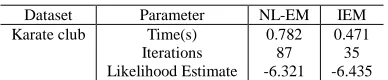
[image:8.595.210.404.721.761.2]

Next, after our IEM algorithm correctly partitions the nodes into two communities, we compare our IEM with baseline algorithm NL-EM. The compared result is shown as Table 1. As we can see from Table 1, under the same computing environment the time of IEM need only 0.471 second, which is much less than it of NL-EM; the iterations of IEM is only 35, which is greatly less than it of NL-EM. From the table we have the following observations. On the dataset, among the two algorithms (NL-EM and IEM), IEM outperforms NL-EM. In other words, our IEM can reach the neighborhood faster than NL-EM, and is high efficient because of fast convergence rate.

Table 1.The comparison between NL-EM and IEM

Dataset Parameter NL-EM IEM Karate club Time(s)

Iterations Likelihood Estimate

0.782 87 -6.321

CONCLUSION

Community detection is a challenging research problem with broad applications. In this paper we have described an incremental EM method-IEM for community detection. IEM uses the machinery of probabilistic mixture models and the incremental EM algorithm to generalize a feasible model fit the observed network without prior knowledge except the networks and the number of groups. The method is more efficient than previous NL-EM, making use of a new incremental approach which is more close to the optimal solutions. We use only a subset rather than the entire networks allows for significant computational improvements since many fewer data points need to be evaluated in every iteration. We also argue that one can select the subsets intelligently by appealing to EM’s highly-appreciated likelihood-judgment condition and increment factor. We have demonstrated the method with applications to some simple examples, including computer-generated and real-world networks. The method’s strength is its efficiency which leads to high convergence rate and good clustering effect.

As part of future work, we plan to extend our framework in two directions. First, our current model only applied on static networks where no temporal analysis is used for evolution study. We are using our model in dynamic networks to detect communities. Second, so far we only considered the link information. In many applications, the content information is also very important. We are investigating how to incorporate content information into our model.

REFERENCES

[1]Girvan M and Newman MEJ. Proceedings of the National Academy of Sciences, 2002, 99(12), 7821-7826. [2]Newman MEJ and Leicht EA. Proceedings of the National Academy of Sciences, 2007, 104(23), 9564-9569. [3] Ramasco JJ and Mungan M. Physics and Society E, 2008, 77(3), 036122.

[4] Mungan M and Ramasco JJ. Journal of Statistical Mechanics: Theory and Experiment, 2010, 4, 04028. [5]Vazquez A. Populations and Evolution, 2008, 77(6), 066106.

[6] Kirkpatrick S, Gelatt CD, Vecchi MP. Optimization by simulated annealing, Science, 1983, 220(4598), 671–680. [7] Duch J and Arenas A. Physical Review E, 2005, 72(2), 027104.

[8] Condon A and Karp RM. Random structures and algorithms, 2001, 18(2), 116-140.

[9] Zhang B.; Zhang S.; Lu G.. Journal of Chemical and Pharmaceutical Research, 2013, 5(9), 256-262. [10] Zhang B.; International Journal of Applied Mathematics and Statistics, 2013, 44(14), 422-430. [11] Zhang B.; Yue H.. International Journal of Applied Mathematics and Statistics, 2013, 40(10), 469-476. [12] Zhang B.; Feng Y.. International Journal of Applied Mathematics and Statistics, 2013, 40(10), 136-143. [13] Bing Zhang. Journal of Chemical and Pharmaceutical Research, 2014, 5(2), 649-659.