and the Max Planck Institute of Economics.
Downloaded from:
Usage Guidelines:
Please refer to usage guidelines at or alternatively
J
ENA
E
CONOMIC
R
ESEARCH
P
APERS
# 2011 – 060
Behavioural patterns in social networks
by
Anna Conte
Daniela T. Di Cagno
Emanuela Sciubba
www.jenecon.de
ISSN 1864-7057
The J
ENAE
CONOMICR
ESEARCHP
APERSis a joint publication of the Friedrich
Schiller University and the Max Planck Institute of Economics, Jena, Germany.
For editorial correspondence please contact [email protected].
Impressum:
Friedrich Schiller University Jena Max Planck Institute of Economics Carl-Zeiss-Str. 3 Kahlaische Str. 10
D-07743 Jena D-07745 Jena
www.uni-jena.de
www.econ.mpg.de
Behavioural patterns in social networks
Anna Contea,b, Daniela T. Di Cagnoc, Emanuela Sciubbad
aMax Planck Institute of Economics, Kahlaische Str. 10, 00745 Jena, Germany
b
University of Westminster, EQM Department, 35 Marylebone Road, London NW1 5LS, UK
c
LUISS University, Viale Romania 32, 00198 Rome, Italy
d
Birkbeck College, University of London, Malet Street, Bloomsbury, London WC1E 7HX, UK
Abstract
In this paper, we focus on the analysis of individual decision making for the formation of social networks, using experimentally generated data. We first analyse the determinants of the individual demand for links under the assumption of agents’ static expectations. The results of this exercise subsequently allow us to identify patterns of behaviour that can be subsumed in three strategies of link formation: 1) reciprocator strategy – players propose links to those from whom they have received link proposals in the previous round; 2) myopic best response strategy – players aim to profit from maximisation; 3) opportunistic strategy – players reciprocate link proposals to those who have the largest number of connections. We find that these strategies explain approximately 76% of the observed choices. We finally estimate a mixture model to highlight the proportion of the population who adopt each of these strategies.
JEL classification: C33; C35; C90; D85
1
Introduction
Individual strategies for network formation can be extremely complex. The main reason for this is that a network differs from a series of bilateral relationships because of the value that accrues to agents through indirect connections: any two economic agents who have to decide whether to establish a social tie take into account not only their own characteristics and the characteristics of the prospective partner but also their (and the prospective partner’s) position in the social network.
The theoretical literature on endogenous network formation has been influenced by two seminal contributions by Jackson and Wolinsky (1996) and Bala and Goyal (2000). Both papers take a game-theoretic approach to the formation of social ties where the main idea is that players earn benefits from being connected both directly and indirectly to other players and bear costs for maintaining direct links. Predicted outcomes are typically not unique. Even for those cases where the stable network architecture is unique (e.g. the star network in information communication models `a la Bala and Goyal or Jackson and Wolinsky), the coordination problem of which agent occupies which position in the network still remains.
In presence of multiplicity of equilibria and coordination problems, it is hardly surprising that most experimental contributions on this topic have highlighted the difficulty in obtaining convergence to a stable network architecture as predicted by the theory.1
Even in absence of coordination, the observed network structures are ultimately the out-come of individual linking decisions. Aim of this paper is to shed some light on the decision process behind any network formation game.
We ran a computerised experiment of network formation, where all connections were beneficial and only direct links were costly. The network formation protocol that we adopted required that links should not be unilateral, but have to be mutually agreed in order to materialise. In particular, players simultaneously submitted link proposals, but a connection was made only when both players involved agree. We ran 9 sessions, with each session involving 6 participants and a minimum of 15 rounds of network formation.
Using the data so generated, we first tried to understand each player’s strategy for network formation through an analysis of the determinants of link proposals. For this purpose, we estimated a system of equations that modelled each player’s decision on the opportunity to propose a link to any of her prospective partners in each round of the game. Relying on the results of such an analysis, we were able to categorise players’ systematic behaviour into
1To be more specific, while convergence may be more easily achieved in experimental settings where the
myopic best response type and opportunistic type. We then verified from our data whether the identified strategies were well represented. Finally, in order to discriminate among these three types of systematic behaviour, we estimated a mixture model to verify if these strategies were well identified and separated in our sample.
The paper proceeds as follows. Section 2 describes the experimental design: the model and the experimental procedure. Section 3 presents and discusses the results of the model of link proposals described in Appendix A. Section 4 shows the characteristics of the three behavioural types that emerged from the analysis in Section 3. Section 5 analyses the data on the light of these three behavioural types. Section 6 develops the mixture model, and Section 7 concludes. The econometric model of link proposals is explained in Appendix A. The instructions (in their English translation) can be found in Appendix B. The software used for the experiment is available from the authors upon request.2
2
The Experimental Design
2.1 The Model
We model network formation as a non-cooperative simultaneous move game. As in Goyal and Joshi (2006), we assume that players’ strategies are vectors of intended links and that links are only formed when they are mutually agreed, i.e. desired by both parties involved. There are positive network externalities in that both direct and indirect connections are beneficial; however direct links are costly.
Consider a set N of n ≥ 3 players, indexed by i = 1,2, ..., n. Each player i submits a vector of intended links:
si = (si1, si2, ..., sin)
An intended link is sij =−1,1 where sij = 1 means that playeri intends to link to player
j while sij = −1 means that playeri does not intend to link to player j. A link between i and j is formed if and only if sij = sji = 1. We denote the formed link by gij = gji = 1, while we represent the fact that there is no mutually agreed link betweeniand j by setting
gij =gji= 0. A strategy profile for all players
s= (s1, s2, ..., sn)
induces an (undirected) network of links g = {gij}i,j∈N, where players are nodes and links
are the edges between them. We say thatiandj are connected in the graphg if there exists a path of adjoining nodesk1, k2, ..., km such thatgik1 =gk1k2 =...=gkm−1km =gkmj = 1.
2The software utilised for the experiment has been developed by InformaRoma. We are especially grateful
Denote by ndi the number of direct neighbours of player i, and by ni the number of his direct and indirect connections. More in detail, denote byndi the number of elements of the setNid={j|gij = 1} and byni the number of elements of the set Ni ={j |there is a path ingfromitoj}.Notice that ifiand jare directly linked, then there is a path between them (of length 1): hence necessarilyni ≥ndi. Player i’s payoff, given his position in the network
g, is assumed to be equal to:
πi(g) =b·ni−c·ndi,
wherebandcare non-negative constants that represent, respectively, the unitary benefit from (direct and indirect) connections and the unitary cost of direct links.
Players aim at maximising their payoffs and may rationally form new links or sever ex-isting ones for this purpose. Goyal and Joshi (2006) characterise equilibrium networks by introducing the notion of pairwise equilibrium networks. A pairwise equlibrium network is such that there exists a Nash equilibrium strategy profile that induces the network (so that no agent has any incentive to deviate from his current vector of intended links) and such that no pair of agents have any incentive to form a new link. More in detail, for any two agents who are not linked in a pairwise equilibrium network, if one of them gains by establishing a new link, it must be the case that the other agent is made strictly worse off by the new link. Formally:
Definition: A network g is a pairwise equilibrium network if the following conditions hold:
1. there is a Nash equilibrium strategy profile (s∗i, s∗−i) that induces g;
2. for gij = 0,if πi(g+gij)−πi(g)>0 then πj(g+gji)−πj(g)<0
Goyal and Joshi show that all Nash networks are minimal. A minimal graph is such that there is at most one path connecting any two agents: there are no redundant links. The intuition why this has to hold is that if there are redundant links, then there are agents who can be reached both directly and indirectly. Agents could obtain higher payoffs by deleting their (costly) direct links to all those nodes that they are able to reach indirectly through others.
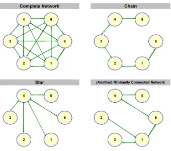
As long as b > c >0, all pairwise equilibrium networks are both minimal and connected (or minimally connected), i.e. there is one and only one path connecting any two agents.3 The intuition behind this is that if there is any isolated node, given that the benefit from an extra connection is higher than the cost of a direct link (b > c), then there are incentives for a new link to be formed between the isolated player and at least another node in the graph. The complete network, where every node is directly connected to every other, is an ex-ample of connected graphs. The complete network is clearly not minimal as there are many redundant links. Examples of minimally connected graphs are the star and the chain.
Figure 1: Examples of network architectures.
2.2 The Experimental Procedure
The experimental sessions were conducted in spring 2006 at CESARE, LUISS University in Rome with a total of 54 participants. Subjects were first-year Economics students. Each subject participated in only one session and none had previously taken part in a similar experiment. We ran 9 computerised experimental sessions with 6 participants each. Each experimental session lasted between 30 and 45 minutes. Subjects’ total earnings were de-termined by the sum of the profits in each round and were paid using a conversion rate of 100 points per euro. They earned approximately 27 euros on average, on top of a 5 euros participation fee.
We implemented a single treatment, for which detailed parameters are given in the table below:4
Participants Initial Endowment Cost Benefit Sessions 1 - 9 6 500 90 100
All relevant parameters were equal across participants and displayed on the screen at all time throughout the experiment.
At the beginning of each session subjects were told the rules of conduct and provided with detailed written instructions, which were read aloud by the experimenters.
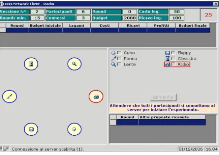
Sessions consisted of a minimum of 15 rounds, with a random stopping rule determining the end of the experiment.5 In each round, subjects were asked to submit (anonymously and independently) a vector of intended links. The initial screen for each participant is shown in
4For an aggregate analysis of the experimental results obtained in this and two alternative treatments,
where the role of the unitary cost of link formation was explored, see Di Cagno and Sciubba (2008).
5At the end of round 15 (and of each additional round after that), a lottery administered by the computer
Figure 2: The initial screen.
Figure 1a.
Participants were represented on the screen by different symbols which we considered neutral in that they did not provide subjects with any particular clue when deciding to establish a link with another player in the group.6 Subjects did not know their symbol (or the other participants’ symbols) in advance and could identify themselves on the screen because their symbol was circled in red. In order to guarantee not only individual but also group anonymity, participants were invited to the lab in groups of eighteen, with three sessions being carried out at the same time. Participants were not told in which of the three groups of six they were playing, nor could they identify the group from their seating.
The screen also displayed the relevant parameters for the session at play. After all sub-jects had confirmed their choice of network partners, the computer checked which links were mutually desired and activated them. At the end of each round, profits were computed and displayed on the screen. Great care was taken in making sure that all available information was provided to the experimental subjects in a user-friendly way. For this reason the graphical interface was designed such that actual links were visualised on the screen as a graph rather than a list of activated ties or as a matrix of−1/1 connections.
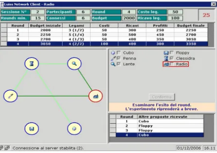
As an example, Figure 1b shows the players’ screen at the end of round number 4. It displays the graph of all active links, total revenues, costs and profits in the round. It also provides information on past unmatched proposals: at the end of a round each subject was informed of those players who proposed a link to them but to whom they did not reciprocate. At any time during the experiment, subjects had access to a great deal of information on past history: by clicking on the bar corresponding to each round, they were able to visualise the graph of active links and the profits obtained in that round.
6In this setting we wanted to avoid any salient coordination device that induces coordination in a particular
Figure 3: An example of the participants’ screen at the end of a round.
3
The Model of Link Proposals
The emerging network structure at the end of each round represents players’ linking decisions. In this section, we analyse and discuss the determinants of link proposals. In doing so, we make the assumption of players having static expectations; that is, we assume that each player myopically expects her co-players to make exactly the same choices in round t as in roundt−1. In some sense, a myopic perspective is induced by the design of the experiment itself: the networks that result from choices in previous rounds are portrayed on the computer screen together with all the relevant information and made accessible throughout the game.
Using the system of equations described in Appendix A, we estimate the probability of each subject i proposing a link to any of his prospective partners j, with j = 1, . . . ,5, as a function of the position of i and j in the network reached in the previous round, which is represented graphically on the subject screen. More in detail, we estimate the probability of subjects proposing a link as a function of a number of variables that can be classified into four categories: the characteristics of the relationship proposer-recipient, which, in particular, include the lagged dependent variable; the characteristics of the prospective-partner; the characteristics of the proposer herself; the characteristics of the network of links observed in the previous round. We also control for experience.
3.1 Estimates Results
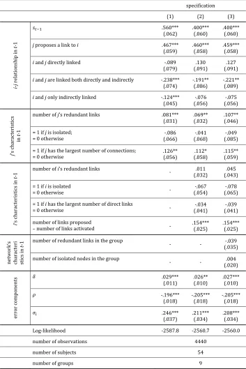
The estimates results of the 5-equation multivariate dynamic probit model derived in Ap-pendix A are reported in Table 1.7
First of all, we can observe that the coefficient on the lagged dependent variable, st−1, is
positive and strongly significant. This suggests that subjects tend to build on what they did in the previous round and therefore vindicates our reasons for studying individual behaviour in a network formation game from a myopic viewpoint. Concerning the relationship between
i and her co-player,j, it seems more likely that a link is proposed if the recipient demanded a link to the proposer in the previous round, thus showing a strong propensity to reciprocate. There is also some evidence on the tendency to cut redundant links since the probability of proposing a link seems to diminish ifiandjwere previously linked both directly and indirectly and also if they were linked only indirectly, even if not in terms of all the specifications of the model. The fact of iand j being linked directly plays no role here. These results make us conclude that, while the propensity to reciprocate demanded links is predominant among players, cutting redundant links might be limited instead to only part of the players and that the remainder might not be particularly concerned about efficiency.
The results regarding the probability of iproposing a link toj as a function of j’s char-acteristics are in support of a hypothesis that sees some of the players acting in a rather opportunistic way. In effect, they appear to look for links that might guarantee them to be connected with the largest number of nodes.8 This follows from our observation that players tend to propose links to those who have the largest number of connections and that demanding a link is more likely, the larger the number of the co-player’s redundant links – an indicator of high connectivity. If a player is instead isolated – that is, she has no connection of any sort – the other players do not seem to be willing to include her.
Among the variables that describeiin the previous round, we find strong evidence of the fact that the propensity to demand a link increases only if the breakdown rate in the previous round – measured as the difference between the number of links proposed and the number of links activated – increases.
We also estimate the propensity to propose a link as a function of the characteristics of the network of links that emerged in the previous round. Despite the large number of variables representing the network structure tested, none of them seem to play a significant role in subjects’ decision. An example is reported in the third column of Table 1. It shows that neither the coefficient on the number of redundant links nor that on the number of isolated nodes in the group are statistically significant. We therefore conclude that players
7
We have estimated several specifications of the model of link proposals, using many combinations of parameters and interaction terms as well as different proxies to represent subjects’ and networks’ characteristics. In Table 1, we report the selection of results that, in our opinion, gives the clearest picture of the main findings. All other results are available from the authors on request.
8
specification
(1) (2) (3)
i ‐ j relationship in t 1 .560***
(.062) .400*** (.060) .400***(.060)
j proposes a link to i .467*** (.059)
.460*** (.058)
.459*** (.058)
i and j directly linked ‐.089 (.079)
.130 (.091)
.127 (.091)
i and j are linked both directly and indirectly ‐.238***
(.074) ‐.191** (.086) ‐.221**(.089)
i and j only indirectly linked ‐.124*** (.045) ‐.076 (.056) ‐.075 (.056) j ‘s characteristi cs in t 1
number of j’s redundant links .081*** (.031)
.069** (.032)
.107** (.046)
= 1 if j is isolated;
= 0 otherwise (.066)‐.086 (.068) ‐.041 (.085) ‐.049
= 1 if j has the largest number of connections;
= 0 otherwise .126** (.056) (.058) .112* .115** (.059)
i
‘s characteristics in
t
1 number of i’s redundant links ‐ (.032) .011 (.043) .045
= 1 if i is isolated
= 0 otherwise ‐ (.054) ‐.067
‐.078 (.065)
= 1 if i has the largest number of direct links
= 0 otherwise ‐ (.041) ‐.034 (.041) ‐.039
number of links proposed
– number of links activated ‐ .154*** (.025)
.154*** (.025)
network‘s characteri stics i
n
t
1 number of redundant links in the group ‐ ‐ ‐.039
(.035)
number of isolated nodes in the group
‐ ‐ (.020) .004
error compone
nts .029*** (.011) .026** (.010) .027*** (.010)
‐.196*** (.018) ‐.205*** (.018) ‐.205*** (.018) .246*** (.037) .211*** (.034) .208*** (.034)
Log‐likelihood ‐2587.8 ‐2560.7 ‐2560.0
number of observations 4440
number of subjects 54
number of groups 9
[image:11.612.125.478.99.628.2]
Table 1: Estimates results of three specifications of the model of link proposals detailed in Appendix A. The coefficients on the group fixed effects,λg, are omitted.
are incapable to take into account the global structure of the network established in the previous round when expressing their willingness to demand a link and choosing the receiver of that proposal.
Table 1 also shows that the correlation coefficient ρ is precisely estimated to be about −.20. It is also significantly different from zero and negative, as expected. This indirectly supports our reasons or dealing with individual link proposals as being jointly determined. The considerable magnitude of the standard deviation of the individual-specific propensity to demand links, σα, puts into evidence the heterogeneity of the population. Finally, the coefficientδis estimated to be positive and significantly different from zero, so indicating that the noise diminishes, the higher the level of experience that players accumulate by playing the network game for several rounds.
As stated earlier, this exercise was meant to search for the leading motives of individual linking decisions. In effect, our analysis has identified the three main drives of players’ choices: a widespread attitude to reciprocate demanded links, efficiency concerns and opportunistic designs.
Given these results, we expect to find at least three patterns of behaviour in our sample:
• players who act by simply reciprocating link proposals from the previous round;
• players who reciprocate to those who demanded a link in the previous round unless they can be reached otherwise through indirect connections (this behaviour corresponds, in fact, to profit maximisation);
• players who try to reach the largest number of nodes by reciprocating to those who exhibit a high connectivity.
In what follows, we will try to establish whether these patterns of behaviour are effectively adopted by players in our sample and, if so, whether there are players who systematically follow one of these patterns.
4
Strategies of Link Formation
In each round of link formation, individuals have 32 available strategies. For each player, a strategy is given by a 5-dimensional vector of 0s and 1s. For example, a possible strategy of player 1 is to propose a link to each of the other 5 players in the game:
(1,1,1,1,1)
the same strategy in roundtthat they played in roundt−1. Hence, given these expectations on what the others will play, each player responds by selecting one of the strategies in the strategy set. In order to understand whether the behavioural patterns defined in the previous section are in fact represented in our sample, we have to define the specific characteristics required of a strategy such that it pertains to a specific behavioural type. The strategies eligible to be assigned to a type are the following:
• A strategy is of reciprocator type if it allows to reciprocate to all the link proposals received in the previous round;
• A strategy is of myopic best response type if it maximises player’s profit, given what the others did in the previous round;
• A strategy is of opportunistic type if it allows to reciprocate to all the link proposals received from those who have achieved the largest number of connections.
The strategies that fit our behavioural types are typically not unique. For example, if the target of reciprocators and opportunists is, for the former, to positively respond to link proposals and, for the latter, to reciprocate to link proposals in order to (indirectly) maximise their own connections then proposing or not proposing additional links is indifferent to the achievement of their primary target. Similarly, for a myopic best responder there will be more than one strategy that maximises profits. In fact, in a myopic setting, if player 2 did not propose a link to player 1 in the previous round, player 1 will be indifferent between proposing or not proposing a link to player 2 in the current round. Given that link proposals need to be reciprocated for a link to be activated, proposing a link to someone who does not reciprocate to you yields exactly the same outcome as not proposing any link, rendering it indifferent to profit maximisation.
It is worth noting that there are less trivial ways in which players may be indifferent between multiple best responses: suppose that in the previous round all other players were connected to each other and to player 1 so that a complete network could be observed. Any of the following one-link strategies is a best response for player 1:
(1,0,0,0,0) (0,1,0,0,0) (0,0,1,0,0) (0,0,0,1,0) (0,0,0,0,1)
In other circumstances, a player’s best response could be strict (i.e. unique). Suppose that in the previous round the observed network is a star where player 1 is the hub: all other players propose links to player 1 and player 1 only. In the current round, the best response of player 1 is unique and it consists of proposing to all other players:
Finally, if player 1 was not offered any link in the previous round, then any of the 32 strategies is a best response. By the same token, in a similar situation all the 32 strategies account for as both reciprocators’ and opportunists’ choices.
5
Analysis of Experimental Data and Behavioural Types
In this section, we analyse the experimentally generated data in light of the behavioural types defined in the previous sections in order to verify whether the strategies, as defined in the previous section, are represented in our sample.
In our experimental sample, 331 out of 888 (37%) of the individual choices appear as if
they were made by reciprocators. In order to assess whether this is a high percentage of choices or not, we decided to compare it to the proportion of times a player who selects a strategy at random ends up selecting a reciprocator strategy. This comparison is particularly useful in our framework where the set of strategies at a reciprocator’s disposal contains more than one strategy. Assume, for example, that in a typical round the experimental network that has been formed is such that for the next round half of the available strategies are of the reciprocator type. In that case, even someone choosing a strategy at random would have a very good chance of selecting a reciprocator strategy.
For sake of comparison, we assume that all participants select strategies at random, with each of the 32 strategies having a probability equal to 1/32 of being selected. Under this assumption, we simulate 1000 samples with the same number of sessions, rounds and partic-ipants as in our experiment.
Figure 4 shows the histogram of the proportion of reciprocator choices from the simulated samples. Such proportions range from a minimum of 0.175 to a maximum of 0.265 with a mean and a median of 0.22 and a standard deviation of 0.01. In the graph, a vertical line representing the proportion of best responses in the real sample is superimposed. We observe that it is considerably above the whole distribution of the proportion of best responses under the hypothesis that all individuals are playing at random. This result suggests that experimental subjects reciprocate intentionally.
Having established that a significant share of choices in our experiment correspond to a ‘deliberate’ desire to reciprocate, we repeat the exercise with the other two types.
0 10 20 30 40 De n s it y
.15 .2 .25 .3 .35
Proportion of reciprocator strategies in simulated samples
0 10 20 30 De n s it y
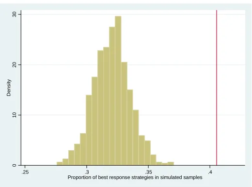
.25 .3 .35 .4
[image:15.612.172.433.103.297.2]Proportion of best response strategies in simulated samples
Figure 4: Histogram of the proportion of reciprocator choices from 1000 simulated samples, where each sub-ject plays a random strategy. The vertical line represents the proportion of reciprocator strategies in the real sample.
0 10 20 30 40 De n s it y
.15 .2 .25 .3 .35
Proportion of reciprocator strategies in simulated samples
0 10 20 30 De n s it y
.25 .3 .35 .4
Proportion of best response strategies in simulated samples
[image:15.612.173.433.425.618.2]
0
10
20
30
De
n
s
it
y
.2 .25 .3 .35 .4 .45
[image:16.612.172.432.75.268.2]Proportion of opportunistic strategies in simulated samples
Figure 6: Histogram of the proportion of opportunistic choices from 1000 simulated samples, where each subject plays a random strategy. The vertical line represents the proportion of opportunistic strategies in the real sample.
0.35 with a mean and a median of 0.31 and a standard deviation of 0.01, compared to 40% in our experimental sample; the proportion of opportunistic choices varies instead between 0.275 and 0.32 with a mean and a median of 0.273 and a standard deviation of 0.012, compared to 44% in our experimental sample.
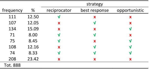
Many choices can be explained by more than one strategy at a time: there are instances when the reciprocator strategy coincides with a best response, an opportunistic strategy or both; there are other instances when reciprocator and opportunistic strategies coincide, or do not coincide, with best response behaviour, and so forth. Table 2 shows the overlap between the strategies arising from our experimental sample.9 The table shows that 40% of all choices can be ascribed to only one behavioural type, the remainder being explained by none of the three types, two types at a time or three. It also shows that almost 77% of all choices in our experimental sample can be explained in the light of one of our three behavioural types. This is quite a high proportion considering that in many cases playing a certain strategy in such a game might be rather difficult.
6
The Mixture Assumption
As seen in the last section, patterns of behaviour often overlap so that the choice of a particular strategy is compatible with more than one behavioural rule. For this reason, discriminating
9In table 2, the first row shows, e.g., that 111 (12.50%) choices in the experimental sample can be accounted
111 12.50 √ x x
107 12.05 x √ x
134 15.09 x x √
71 8.00 √ √ x
75 8.45 √ x √
108 12.16 x √ √
74 8.33 √ √ √
208 23.42 x x x
Tot. 888
[image:17.612.151.454.75.216.2]
Table 2: The table shows the frequency of choices in our experimental sample explained by each of the three strategies alone and all possible overlaps. The green tick indicates when a strategy is represented; the red x when it is not.
between subjects according to their behavioural type is rather difficult if one merely observes the strategies selected by them. In this Section, we want to verify whether subjects system-atically adopt one of the three patterns of behaviours under investigation so that the former can be framed alternatively within our definitions of the reciprocator type (RC), the best response type (BR) and the opportunistic type (OP). In order to assign subjects to these types, we estimate a mixture model (see McLachlan and Peel (2000)) that will allow us to verify if these strategies are well identified and separated in our sample.
We proceed by assuming that a proportion πRC of the population from which the ex-perimental sample is drawn behaves according to the reciprocator type; a proportion πBR behaves according to the best response type; and finally a proportionπOP = 1−(πRC+πBR) behaves according to the opportunistic type. Our mixture assumption is that each subject belongs to one of these types and that she cannot switch type across rounds. The parameters (πRC, πBR, πOP) are known as the mixing proportions and are estimated along with the other parameters of the model.
The likelihood contribution of subject ithen is:
(1) Lig =πRC×lRCig +πBR×lBRig +πOP ×lOPig ,
wherelRC
ig ,lBRig and lOPig are the likelihood contributions of individualiunder the hypothesis of her belonging to the reciprocator type, the best response type and the opportunistic type, respectively. These are derived as follows.
specification
(1) (2) (3)
ߛோ CC CC GFE
ߛோ CC GFE GFE
ߛை CC CC GFE
ߨோ (.088).402 (.080).369 (.080).319
ߨோ (.096).365 (.085).434 (.088).450
ߨை (.072).233 (.064).197 (.070).231
Log‐likelihood ‐518.9 ‐490.3 ‐478.8
observations 888
number of subjects 54
[image:18.612.181.421.74.284.2]number of groups 9
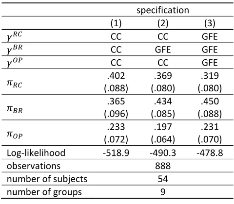
Table 3: Estimates results of the mixture model. CCindicates that a common constant is estimated;GF E
indicates that group fixed effects are estimated. The results are omitted. All mixing proportions are statistically significant at 1% level.
players are more likely to adopt a strategy if there are other players in her group of the same type. Thus individual i’s propensity to choose one of the strategies that correspond to type
his:
yhig,t∗ = γgh+εhig,t i= 1, ...,6 g= 1, ...,9 t= 1, ..., Tg (2)
εhig,t ∼ N[0,1]
Here, εig,t is an error term, distributed standard normal and independent of anything else in the model. yhig,t∗ is a latent variable representing player i’s attitude to act according to strategic type h. The available data is an unbalanced panel since the number of rounds in each session (Tc) depends on a random stopping rule that decides, after round 15, whether or not to continue with another round of the game.
The observational rule is the following:
yig,th = 1 ifsig,t complies with type h’s behavioural rules
yig,th = −1 otherwise
The likelihood contribution of subjecti, conditional on being of type h, is
(3) lhig =Lhigγgh |sig,1, ..., sig,Tg
=Tg
t=1 Φ h
yig,th ×γghi,
[image:19.612.173.430.76.306.2]
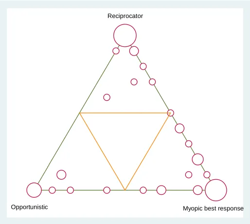
Myopic best response Opportunistic
Figure 7: Posterior probability of types from estimates results in Table 3, specification 2.
Results are displayed in Table 3. In specification 1, where allγgh, withh∈(RC, BR, OP), are estimated as common constants, we find that the predominant type is the reciprocator type, followed by the best response and the opportunistic type. Adding group fixed effects to the best response type significantly increases the log-likelihood according to the likelihood-ratio test (χ28 = 57.2,p-value< .0001), which it does not if added to the other two types. This makes the best response type the most popular with a mixing proportionπBR=.43, followed by the reciprocator type with a πRC = .37 and the opportunistic type with a πOP = .20. Adding group fixed effects to the other two types (reciprocator and opportunistic) does not improve the fit any further (likelihood-ratio statisticχ216= 23, p-value=.1137). Compatible with these results, we observe that doing best response seems group-driven – players are more likely to best respond if they are in a group where there are other players who do best response – whilst playing either a reciprocator or an opportunistic strategy does not depend on what the other players in the group are doing.
Having estimated a mixture model, one obvious thing to do is to compute the posterior probabilities of each experimental subject being of each type. Using Bayes’ rule we have the following posterior probabilities:
Pr [iis of type h|sig,1, ..., sig,Tc] =
Pr [type h]×Pr [sig,1, ..., sig,Tc |type h] Pr [sig,1, ..., sig,Tc]
= πh×Pr [sig,1, ..., sig,Tc |type h] Pr [sig,1, ..., sig,Tc]
= πh×l h i
forh∈ {RC, BR, OP}.Posterior probabilities are reported on the simplex displayed in Figure 7. The 54 subjects are represented by circles in the graph: small circles represent a single subject; larger circles cluster subjects concentrated in that area of the simplex (the larger the circle the more numerous the cluster). The closer a subject is to a vertex of the simplex the greater the posterior probability for that subject of being of the type represented on that vertex.10 Subjects in the bottom left corner are of the opportunistic type; subjects in the bottom right corner are of the best response type and, finally, those in the top left corner are of the reciprocator type. The vast majority of subjects are located very close to the vertices of the simplex, a minority to the edges and no one is in the middle. The yellow simplex in the centre represents a virtual area of “uncertainty over types” and is empty in the case under examination. This finding confirms that the mixture model clearly separates the three types of individuals, with most of them being assigned to a particular type with quite a high posterior probability.11
7
Conclusions
In the era of virtual social networks such as Facebook, or LinkedIn, there is very little doubt that network membership is generally seen as a positive ingredient for personal achievement and increased chances of success.
The mesh of interpersonal and community relations which facilitate communication, in-formation and exchange is part of what has been called ”social capital”. This is a nebulous concept and difficult to quantify but it is generally agreed that it strongly affects behaviour and individual outcomes. Given that personal success can be both the result and the pre-requisite of a large social network, any attempt to quantify the impact of social capital on outcomes has to take into account the process of network formation.
For this reason, we focus our paper on individual linking strategies in a network formation game. We use experimentally generated data to this purpose.
By a system of equations modelling players’ decision in each round of the game on their demand of a link to their co-players, we have succeeded in distinguishing between reciprocator strategies, myopic best response strategies and an opportunistic strategies.
We find that approximately 37% of the network formation strategies adopted by the exper-imental subjects can be accounted for as reciprocator strategies, 40% as myopic best response strategies and 44% as opportunistic strategies. Adding reciprocator, myopic best response and opportunistic behaviour, we are able to explain approximately 76% of the observed choices. We show that each of these types of behaviour is ‘deliberate’ in that we have obtained shares of each behaviour that are significantly different from what would have obtained if agents had selected links at random.
10
For producing the simplex, posterior probabilities have been rounded to the closest.05.
assumption can be validated for our sample. We find that it is safe to assume that each individual belongs to one type, with mixing proportions approximately equal to 43%, 37% and 20% for best response, reciprocator and opportunistic types, respectively.
Finally, we observe that the individual attitude to best respond is heavily group driven, with agents being more likely to best respond when others in the same session also do so. This has not happened in the case of reciprocator and opportunistic types.
Why are the findings of our analysis relevant? We argue that our results respond, in some sense, to the recent network formation research that develops equilibria with farsighted agents.12 In fact, the three strategies we have identified and analysed are all based on the assumption of static expectations on what the rest of the group will do and they are alone able to explain the most part of subjects’ behaviour in network formation. We do not pretend to affirm that there are no farsighted agents in the population, but that a myopic approach still deserves attention.
12
Appendix A. The econometric model of link proposals
In each round of the game, each subject submits a vector of choices concerning the opportunity to propose or not propose a link to any of her co-players. From a player’s perspective, the decision to propose a link to one of her co-players is not separate from the decision to propose or not propose a link to another co-player. For this reason, all decisions made by a player in a round are not independent but they are the result of a joint evaluation and need to be analysed as such.13
Let us consider a set of 6 players, indexed byi= 1, . . . ,6. Each playeri in roundt submits a 5-dimensional vector of intended links:
sig,t= (si1g,t, . . . , sijg,t, . . . , si5g,t).
Here, j = 1, . . . ,5 represents i’s prospective players; groups of co-players are indexed by g, withg= 1, . . . ,9;t= 2, . . . , Tgindicates the round number. The final round number,Tg, may differ by group because of a random stopping rule that decides, after round t= 15, whether or not to continue with another round of the game. sijg,t equals 1 if subject i expresses his willingness to be linked toj; it equals−1 otherwise.
The vector of intended links sigt is the result of a complex decision process. In making her decisions, i needs to jointly evaluate the opportunity to propose a link to each of her 5 prospective players. In other words, ineeds to consider the following system of equations:
s∗ijg,t = (1 +δ(t−2))×
αi+λg+β
0
wWijg,t−1+β
0
xXjg,t−1+β
0
yYig,t−1+β
0
zZg,t−1
+uijg,t,
for j= 1, . . . ,5 and j 6=i.
(5)
Here, Wijg,t−1 is a vector of explanatory variables describing the characteristics of the
re-lationship between i and j in the previous round, including the lagged dependent variable,
sijg,t−1;Xjg,t−1 is a vector of characteristics ofjas shown by the network that emerged in the
previous round; Yig,t−1 is a vector of explanatory variables related to i’s position in the
net-work in the previous round; the explanatory variables in Zg,t−1 describe the main features of
the network resulting from players’ link proposals in the previous round. There are also two regression intercepts, αi and λg. Intercept αi varies across individuals (individual-specific time-invariant random effect) and is assumed to be common to all equations in (1). We also assume that it does not depend on any observable. It represents the individual-specific propensity to demand links and is assumed to be distributed normal across the population:
αi ∼N 0, σα2
. In a network formation game, individual decisions within a group may well
13Cf. Di Cagno and Sciubba (2008), who disregard this characteristic of players’ decisions, deal with each
– for example, because all individuals observe the same sequence of graphs occurring during a session. Our method of controlling for dependence on unobservables within a session is to model the intercepts λg as random unobservables (group-specific fixed effects). The term (1 +δ(t−2)) is introduced in order to capture the effect of experience on players’ decisions. A positive (negative)δ implies that subjects’ choices eventually become less (more) noisy.14
s∗ijg,t– the latent dependent variable representing subject’sipropensity to demand a link toj
– andsijg,t, the observed binary outcome variable, are related by the following observational rule:
sijg,t=
(
1 ifs∗ijg,t≥0
−1 else .
Since players in each round jointly evaluate the opportunity to propose a link to any of their co-players, we expect that the choice of proposing a link to one of the prospective partners reduces the probability of proposing a link to the others. In other words, we expect to observe a negative correlation across the equations in (1).15 i’s decision in each round can be framed within the class of M-equation multivariate dynamic probit models. Anyhow, we need to place some restrictions on the variance-covariance matrix of the errors and the coefficients on the system’s variables. In particular, the joint distribution of the error terms is assumed to take the form:
V
ui1g,t .. .
uijg,t .. .
ui5g,t
=
1 · · · ρ · · · ρ
..
. . .. ... ... ...
ρ · · · 1 · · · ρ
..
. . .. ... ... ...
ρ · · · ρ · · · 1
. (6)
Here, error variances on the leading diagonal of V have values of 1 and the off-diagonal
elements are all equal to ρ. This hypothesis of equi-correlation of the error terms of the system of behavioural equations (1) follows from the fact that there is no reason to assume that a certain pair of equations in (1) are more or less correlated than another pair. Further, we assume that the coefficients on the variables in system (1) do not vary across equations.
Estimation of the dynamic system (1) requires an assumption about the initial
obser-14A positive δwould eventually reduce the error variance (that is constrained to be equal to 1 in round 2
for identification purposes), consequently making the role of the stochastic disturbance less and less relevant in players’ decisions and, in this sense, highlighting the role of experience accumulated throughout the game.
15
vations sijg,1. Since players do not know anything about their co-players and the group of
players as a whole before the graph of the network resulting from round 1 link proposals is shown to them, we can safely assume that the initial conditionsijg,1 is completely random.
Let us define playeri’s likelihood contribution as:
Lig =
Z ∞
−∞
Tg
Y
t=1
Φ5(µig,t; Ω)f α; 0, σ2α
dα,
(7)
where µig,t= (si1g,t×µi1g,t, . . . , sijg,t×µijg,t, . . . , si5g,t×µi5g,t) and µijg,t= (1 +δ(t−2))×
αi+λg+β
0
wWijg,t−1+β
0
xXjg,t−1+β
0
yYig,t−1+β
0
zZg,t−1
, with j = 1, . . . ,5; Ω is a sym-metric 5 ×5 matrix whose elements on the leading diagonal are equal to 1 (σjj = 1 for
j = 1, . . . ,5) and are equal toσjk =sijg,t×sikg,t×ρ(forj, k= 1, . . . ,5 andj6=k) somewhere else; f α; 0, σ2α is the normal density function with mean 0 and varianceσ2α evaluated atα. The multivariate normal cumulative distribution function Φ5(.) is evaluated by the
Geweke-Hajivassiliou-Keane (GHK) algorithm.16 The likelihood function is maximised using 20-point Gauss-Hermite quadrature.17
16
This is implemented in Stata 12 by themvnp()function; see Cappellari and Jenkins (2006).
Welcome
This is an experiment on the formation of links among different subjects. If you make good choices you will be able to earn a sum of money that will paid to you in cash immediately after the end of this session.
You are one of 6 participants to this experiment; at the very beginning the computer will randomly assign to you an initial budget (equal across participants). The computer will also randomly assign to you an icon (Dropper,Radio,Cube,Floppy disk,Hand lens,Hour glass) that will identify you throughout the experiment and will assign you an initial budget (equal across participants). The icon identifying you is circled in red on your screen.
The experiment consists of a random number of rounds: there will be at least 15 rounds, after which a lottery administered by the computer will determine whether there will be a further round or the experiment is over.
Each participant to this experiment represents a node. At the beginning of the experiment all nodes are isolated. In each round, the computer will ask you whether you want to propose any link and to whom. You may propose 0, 1 or more links. The computer will collect the proposals from all participants and activate only the links desired by both of the two subjects involved (reciprocated proposals).
Your screen will show the graph of active links. The box at the bottom right corner of your screen will show you who has proposed a link to you in the previous round and to whom you have not reciprocated.
Each link that you manage to activate has a cost (equal across participants) that is indicated on the screen. In each round, the computer may reject your link proposals if they entail an expenditure that is higher than your budget for that round.
Your revenues in each round are automatically computed and are given by the product by the revenue per node (equal across subjects and indicated on your screen) and the number of nodes that you manage to reach both through your direct links and the links activated by other participants.
Computing costs and revenues
Example: subject Radio is directly linked to Floppy disk and Dropper and indirectly, that is throughDropper, toHand lens.
In each round, the computer calculate out your profit and display it on your screen. The overall profit from the experiment is given by the sum of your revenues in all rounds. At the end of the experiment, you will be paid in cash an amount in euros equivalent to 10% of your total profit.
At the beginning of the experiment please wait for instructions from the experimenters before touching any key.
When the experimenter asks you to do so, please double-click only once on the “Network Client” icon on your desktop.
The following screen will appear:
The screen gives you all the information regarding the round that you are about to play. Be careful: each round has a maximum time duration given by the number of seconds indicated in red at the top right corner of your screen. If you have not managed to make your choice by then, the computer will immediately proceed to the next round.
Your screen shows all the relevant data useful for the current round (available budget, costs and revenues) as well as the results that you have obtained from each of the previous rounds.
When the message ”Round is now active” appears at the bottom of your screen, you can make your choice by ticking the boxes corresponding to the icons that you want to propose a link to. When you are done, press “Confirm”. When all participants have confirmed their choices, the computer will show the results of the round on the screen.
You will be advised of the beginning of a new round by a ”New Round” message. Be careful: after the 15th round, red and green lights will flash on the screen. If the lights stop on green, you will play another round; if they stop on red, the experiment is over.
It is very important that you make choices independently and that you do not communi-cate with other participants during the experimental session.
At the end of the last round the experiment is over, and you will be paid a sum in cash corresponding to your profit during the course of the whole experiment.
For any problem, please contact the experimenters. Enjoy.
References
Bala,V., Goyal, S., 2000. A Non-Cooperative Model of Network Formation. Econometrica, 68(5): 1181-1229.
Bernasconi, M., Galizzi, M., 2005. Coordination in networks formation: Experimental evi-dence on learning and salience. FEEM Working Paper, 107.
Berninghaus, S.K., Ott, M., Erhart, K.M., 2008. Myopically forward-looking agents in a network formation game: Theory and experimental evidence. Sonderforschungsbereich, 504.
Berninghaus, S.K., Ott, M., Erhart, K.M., Vogt, B., 2007. Evolution of networks - an experimental analysis. Journal of Evolutionary Economics, 17: 317-347.
Callander, S. and Plott, C., 2005. Principles of Network Development and Evolution: An experimental Study. Journal of Public Economics, 89(8): 1469-1495.
Cappellari, L., Jenkins, S.P., 2006. Calculation of multivariate normal probabilities by sim-ulation, with applications to maximum simulated likelihood estimation. Stata Journal, 6(2), 156-189.
Conte, A., Moffatt, P.G., 2011. The econometric modelling of social preferences. mimeo.
Conte, A., Levati, M.V., 2011. Use of data on planned contributions and stated beliefs in the measurement of social preferences. Jena Economic Research Papers, 2011-039.
Deck, C. and Johnson, C., 2004. Link Bidding in Laboratory Network. Review of Economic Design, 8(4): 359-372.
Di Cagno, D., Sciubba, E., 2008. The Determinants of Individual Behaviour in Network Formation: Some Experimental Evidence. M.Abdellaoui and J.D. Hey (eds), Springer, Theory and Decision Library, Cambridge.
Dutta, B., Ghosal, S., Ray, D., 2005. Farsighted network formation. Journal of Economic Theory, 122: 143-164.
Goeree, J.K., Riedl, A. and Ule, A. 2009. In Search of Stars: Network Formation among Heterogeneous Agents. Games and Economic Behavior, 67: 445-466.
Goyal, S., Joshi, S., 2006. Unequal connections. International Journal of Game Theory, 34: 319-349,
Grandjean, G., Mauleon, A., Vannetelbosch, V., 2009. Connections among farsighted agents.
Working Paper, 21.
Herings, P.J., Mauleon, A. Vannetelbosch V., 2009. Farsightedly stable networks. Games and Economic Behavior, 67(2): 526-541.
Jackson, M.O., Wolinsky, A., 1996. A Strategic Model of Social and Economic Networks.
Journal of Economic Theory, 71(1): 44-74.
McLachlan, G., Peel, D., 2001. Finite Mixture Models. Wiley and Sons, New York.