The effects of different parameterizations of Markov switching in a CIR model of bond pricing

effects of different parameterizations of Markov-switching in a CIR model of

bond pricing. Studies in Nonlinear Dynamics & Econometrics 13 (1), ISSN

1081-1826.

Downloaded from:

Usage Guidelines:

Please refer to usage guidelines at

or alternatively

Enabling open access to Birkbeck’s published research output

The effects of different parameterizations of

Markov-switching in a CIR model of bond pricing

Journal Article

http://eprints.bbk.ac.uk/1934

Version: Publisher draft

Citation:

© 2009 Berkeley Electronic Press

Publisher version

______________________________________________________________

All articles available through Birkbeck ePrints are protected by intellectual property law, including copyright law. Any use made of the contents should comply with the relevant law.

______________________________________________________________

Deposit Guide

Volume

13,

Issue

1

2009

Article

1

The Effects of Different Parameterizations of

Markov-Switching in a CIR Model of Bond

Pricing

John Driffill

Turalay Kenc

Martin Sola

Fabio Spagnolo

∗_{Birkbeck College, University of London, [email protected]}

†_{Bradford University School of Management, [email protected]}

‡_{University of London and Universidad Torcuato Di Tella, [email protected]}

∗∗_{Brunel University, [email protected]}

John Driffill, Turalay Kenc, Martin Sola, and Fabio Spagnolo

Abstract

We examine several discrete-time versions of the Cox, Ingersoll and Ross (CIR) model for the term structure, in which the short rate is subject to discrete shifts. Our empirical analysis suggests that careful consideration of which parameters of the short-term interest rate equation that are allowed to be switched is crucial. Ignoring this issue may result in a parameterization that produces no improvement (in terms of bond pricing) relative to the standard CIR model, even when there are clear breaks in the data.

∗_{We thank David Barr, Keith Cuthbertson, Demian Pouzo, Marzia Raybaudi, Daniel Thornton,}

1

Introduction

A popular way of characterizing a process subject to structural breaks is to assume that the breaks follow a Markov chain as in (Hamilton, 1988, 1989). Although an extensive litera-ture uses this approach, few papers systematically study the specification of the switching regression. Questions such as: (i)which parameters are allowed to switch [see Hall and Sola (1993)];(ii)how many states should be allowed for [see (Hansen, 1992, 1996), Garcia (1998), and (Psaradakis and Spagnolo, 2003, 2006)];(iii) how many lags should be included in the switching regression [see Kapetanios (2001)] have attracted comparatively little attention. The importance of each of these questions varies with the application at hand.1 _{The correct}

specification of the switching process is crucial when forecasting, or for applications that involve rational expectations. Different specifications typically imply different forecasts and pricing equations, and consequently affect conclusions about the validity of any theoretical model.

Short and long-term interest rates have been characterized as a stochastic process subject to regime switches [see, for example, Hamilton (1988), Sola and Driffill (1994), Garcia and Perron (1996), Gray (1996), Dahlquist and Gray (2000), Landen (2000), (Ang and Bekaert, 2002a,b), Bansal and Zhou (2002), Smith (2002), Evans (2003), and Dai and Singleton (2003)]. In particular, Gray (1996) showed that a version of the Cox, Ingersoll, and Ross (1985) (CIR) model with time-varying parameters provides an appropriate characterization of US short-term interest rate data. While some of the papers that use the CIR model only allow the volatility of the short-term interest rate to switch [e.g., Naik and Lee (1997)], others, such as Bansal and Zhou (2002), allow all the parameters to switch [see also Dahlquist and Gray (2000) and (Ang and Bekaert, 2002a,b)]. However, none of these papers evaluate the performance of different specifications, either in terms of fit, or in terms of real-time one-step-ahead bond pricing. This paper attempts to fill this gap by evaluating how different parameterizations of the switching process affect bond prices. Therefore, we do not ask, as most of the literature does, which of the many competing models best fit the data in-sample; but, for a given model, what are the effects of allowing all the parameters of the exogenous driving equation to switch (as is standard these days in the literature) on the one step ahead bond prices.2

We rank the different versions of the CIR model in terms of their ability to generate prices close to the data. Our approach is based on recursively estimating the different parameterizations of the switching CIR process, and using the results to price bonds of different maturities. In this way we generate a series of prices which are then compared with the actual prices.3

These results are then compared with those obtained using standard likelihood ratio tests and complexity-penalized likelihood criteria.4 _{We find that the models which provide}

1_{For example, Kim and Piger (2002) found that ignoring some of the dynamics of the output growth does}

not affect, and sometimes even improves, the ability of the filter to correctly separate booms and recessions.

2_{We consider different versions of the CIR short rate process which include: (1) a benchmark case with no}

regime-switching; models with regime-switching in: (2) volatility; (3) volatility and the speed of adjustment; (4) volatility and the long-run value of the short rate; and (5) volatility, the speed of adjustment and the long-run value of the short rate.

3_{To carry out an extensive analysis of the implications of studying the effects of the choice of the}

pa-rameters that are allowed to switch and, more importantly, the relevance of the issue, we use a simple Markov-switching CIR model. We speculate that the point raised in this paper is equally important (or probably more important given the nature of the driving process) for other more complex affine switching models. We explain in detail in the text why we think that this will be the case.

the best fit (and those versions are not rejected by the data) do not necessarily provide the best bond prices. This result seem to suggest that the tendency in the literature to estimate more general and complicated models (with time varying transitions and adding more factors) may simply improve the fit while worsening the one step ahead pricing (which is the main interest of the practitioner) and the forecasting performance of the model [see for example Diebold and Li (2006)].

The main results of the paper are that simpler specifications such as a Markov-switching CIR (MS-CIR) short rate with only regime-dependent volatility and with regime-dependent volatility and long-run interest rate produce better bond prices than those obtained using parameterizations with no regime switching, models where all the parameters are allowed to switch, and parameterizations with both regime-dependent volatility and regime-dependent speed of adjustment. We also find that the pricing gains of Markov-switching models di-minish the further away from the break the bond price is evaluated, to the extent that, eventually, the CIR outperforms the MS-CIR model. Indeed, on the basis of criteria which evaluate the ability of the models to correctly predict turning points (i.e. whether rates are rising or falling), the Markov-switching parameterization may not produce better prices than those obtained using the standard CIR model, even when there are apparent structural breaks in the sample.

The plan of the paper is as follows. In section 2 we present the benchmark model and its extensions which are used to evaluate the empirical issues. Section 3 considers using bond pricing as a model selection criterion for the interest rate. Section 4 summarizes and concludes.

2

Term Structure Models

In this section, we present the Cox, Ingersoll and Ross (CIR) benchmark model that is used to evaluate the alternative empirical issues addressed in the paper. We modify the original CIR model as in Bansal and Zhou (2002) to allow the short-term interest rate to switch between regimes. The benchmark model and its extensions are presented below. Notice that Bansal and Zhou (2002) seem to suggest, that a two factor model has a better fit in sample. Nevertheless, it is not obvious that we can draw any conclusions from their results for our paper since we not only use a different sample period (our data goes up to 1998 instead of 1995) but also, and most importantly, use a different sample frequency. Notice also that there are many differences in emphasis between this paper and that of Bansal and Zhou (2002). First, we study the relative importance of different assumptions which are common in the literature, rather than purposing a new model to explain the term structure. Second, we mostly focus in the out of sample performance of the models rather than trying to explain the model that better prices the past. Third, we the compare full and real sample performance of the different bond prices.

2.1

The Benchmark Cox, Ingersoll and Ross (CIR) Model

We first consider the benchmark CIR model in which a single factorx, typically associated with the short rater, follows a mean-reverting square root process. The discrete-time version of the CIR process for the single factor is written as

xt+1−xt=κ[θ−xt] +σ

√

xtut+1, (1)

with {ut+1} distributed normally, independently, with mean zero and variance one. The

factor reverts to a long-term mean value θ. The parameter κdetermines the adjustment speed ofxtowards the long-term mean, andσ2_{xis the variance of the unexpected changes}

in the factor. The term σ is the local volatility and serves as a scaling parameter. The pricing kernel (stochastic discount factor),M, for a discrete time version of the CIR model is

Mt+1= exp

"

−rf_t −

λ σ

2

xt

2 −

λ σ

√

xtut+1

#

. (2)

We refer toλas themarket price of factor risk, since it determines the covariance between shocks toM andx, and thus the risk characteristics of bonds and related assets. Note that

Et[Mt+1] = exp(−rft), wherer f

t is the one-period risk-free rate. We assume that, for every

τ, the price of a maturityτ-bond has the form:

P_tτ = exp[−Aτ−Bτxt]. (3)

2.2

Regime Shifts

We account for regime switches by assuming that the parametersκ(st),θ(st) andσ(st) in

eq. (1) take different values in different regimes st. We model st as a two-state Markov

process which takes values of either 0 (regime 0) or 1 (regime 1). The switch between the regimes is governed by a Markov chain with a transition probability matrix Π = (πij):

Π =

"

π00 π01 π10 π11

#

, (4)

whereP

j=0,1πij = 1 and 0< πij <1. The probability that a transition occurs from state

st = i (say i = 0) to state st+1 = j (say j = 1) in the interval [t, t+ 1] is equal to π01.

Similarly,πiiis the probability that the process remains in statei. For analytical tractability,

it is assumed that the discrete statesst+1are independent of the random processut+1. It is

also assumed that agents in the financial markets know the actual state of the systemst.5

The Markov-switching mean-reverting square root process (MS-CIR) can be written as follows,

xt+1−xt=κ(st+1)[θ(st+1)−xt] +σ(st+1)

√

xtut+1. (5)

Following Bansal and Zhou (2002) we model the market price of random risk as regime dependent: λ(st+1). The pricing kernel therefore needs to be adjusted for regime shifts as

follows

Mt+1(st+1) = exp

"

−rf_t −

_λ(s t+1) σ(st+1)

2_x t

2 −

λ(st+1) σ(st+1)

√

xtut+1

#

. (6)

5_{However, the econometrician does not observe the actual state and has to make inferences on it based}

2.3

Bond Pricing

We assume that there is a market for every bond at every choice of maturity τ and that the market is arbitrage free. Furthermore, we assume that, for everyτ, the log price of a maturityτ-bond in regimesthas the form

P_tτ(st) = exp [−Aτ(st) − Bτ(st)xt], (7)

whereAandB are deterministic functions.

To ensure that the bond prices satisfy the no-arbitrage condition we use the fundamental pricing equation

P_tτ(st) =Et[Mt+1(st+1)Ptτ+1−1(st+1)]. (8)

We assume that the distribution of the stochastic discount factor Mt+1 is conditionally

lognormal. We specify models in which bond prices are jointly lognormal with Mt+1. We

can then take logs of (8) to obtain

logPtτ(st) =Et[logMt+1(st+1) + logPtτ+1−1(st+1)] +1₂V art[logMt+1(st+1) + logPtτ+1−1(st+1)].

(9) This equation is then used to obtain the constantsAandB,using equations (1), (2) and (3) for the single-regime model and equations (5), (6) and (7) for the switching-regime model. The corresponding solutions are provided, respectively, in appendices A and B. Once the constantsAandB are obtained, bond yields are calculated as follows:

y_tτ(st) =−

logP_tτ(st)

τ =

Aτ(st)

τ +

Bτ(st)

τ xt i= 0,1. (10)

3

Markov-Switching Cox, Ingersoll and Ross (MS-CIR)

Models with Switching Market Price of Factor Risk

In this section we inquire whether a common assumption made in the literature, that all the parameters of the instantaneous interest rate are allowed to switch between regimes, is important for bond pricing. We establish the relative performance of the pricing model under different assumptions about which parameters of the short rate are allowed to switch. In principle overparameterized models might overfit the data and have a poor out-of-sample performance. Since pricing is intrinsically a forecasting exercise (because long term rates are, using the appropriate kernel, some kind of discounted average of the future ex-pected short-term interest rate), we speculate that an overfitted model might also produce ‘bad’ bond prices (i.e., bond prices with big errors).

When using different versions of the single-factor Markov-switching Cox, Ingersoll and Ross model (depending on the assumed switching parameterization) to price bonds, an estimate of the market price of factor risk is required. The parameters λi, (i = 0,1),

measuring the market price of factor risk, are estimated from the data. This strategy is based on a common assumption in the literature where the bond prices are observed with errors for some maturities [see for example Pearson and Sun (1994)]. This allows to jointly estimate the parametersλi along with the other parameters of the model. The yields with

measurement error are given by:

y_tτ= Aτ

τ +

Bτ

In estimatingλi we assume that the yields on bonds with maturities 6 months and 5 years

are measured with error. In this paper we do not impose the assumption that, for the other maturities under consideration (the 1, 2 and 10 years yields), the bonds are exactly observed (priced), but we use those maturities to evaluate the pricing performance of the alternative parameterizations by comparing the prices generated by the model with the actual price. Implicitly we get a measure of how strong is that assumption.

The assumption that some maturities are observed without error, and therefore are exactly priced, has contributed to the increasingly common use of highly parameterized models (i.e. models with several factors, models where all the parameters are allowed to switch and/or models with time varying probabilities). This is because, under the assump-tion that some maturities are observed without error, only complex models can fit the data in the sample. This strategy is usually defended on the grounds that it rules out arbitrage opportunities. Nevertheless we argue that this argument might be misleading because: i) the ex-ante pricing (or out-of-sample forecasting) performance of those highly parameterized models is usually very poor; ii) some of the maturities that are priced without error are, most of the time, synthetic and constructed from coupon paying bonds (that is, the data are by construction only an approximation).

3.1

Comparison Based on Goodness of Fit

For the estimation of the parameters of the model we use the 3 month T-Bill yield as a proxy of the instantaneous rate.6 _{We use quarterly data to avoid the potential serial}

correlation which would be induced by the existence of overlapping expectations whenever the sampling frequency is higher than the maturity of the short term interest rate. The five models specified intable 1 are estimated for the period 1964:1–1998:4, using the 3, 6 month bills and 5 years bond. We use the 1, 2, and 10 year bonds for the evaluation of the models. The estimation of the different models for the short-term interest rate is carried out by using the recursive algorithm discussed in (Hamilton, 1988, 1989). This gives as a by-product the sample likelihood function which can be maximized numerically with respect to Θ = {κ0, κ1, θ0, θ1, σ0, σ1, λ0, λ1,Σ₀,Σ₁}, subject to the constraint that p= P(st+1 =

1|st= 1) andq=P(st+1= 0|st= 0) lie in the open unit interval (see Appendix C).7

Intable 2, we report Gaussian standard pseudo-maximum likelihood (S–PML) estimates of the parameters along with the corresponding asymptotic standard errors.8 _{Given the}

nature of the maximizing algorithm, we need to classify the regimes, not only in terms of the parameters of the switching CIR model, but also in terms of the state dependent variance-covariance matrix of the maturities priced with error. We find that the variances (for both maturities) of the pricing equations for the maturities observed with error in state 0 are higher than those variances in state 1, {σ2

0(6m) > σ 2 1(6m), σ

2

0(5y)> σ 2

1(5y)} (below we

offer an explanation for this finding). We find, for all models, that state 1 is more persistent that state 0,{κ0< κ1}; that the volatility of the short term interest rate is higher in state 1 than in state 0, {σ1 > σ0}; and that (except for model 5) the long run value is higher in state 0 than in state 1,{θ0 > θ1}.9 _{At this stage it should be clear that when many}

6_{The data used in this paper are available on the web page associated with Duffee (2002).} 7_Σ

0 and Σ1 are the variance covariance matrices of the pricing errors for the maturities assumed to be

observed with error in state 0 and 1 respectively.

8_{The likelihood function was maximized by using the Broyden–Fletcher–Goldfarb–Shanno quasi-Newton}

algorithm with numerically computed derivatives.

9_{In the estimation and pricing the interest rates are expressed in quarterly basis (instead of in annual}

pararameters are allowed to switch, even the definition of the regimes is cumbersome. This is aggravated by the fact that the variance-covariance matrix of the pricing error equations also is regime-dependent.10

In figure 1 we plot all the maturities of Duffee (2002) along with the estimated filter probabilities. As explained above, the separation of the filter mostly associates regime 0 (regime 1) with: i) high (low) pricing errors (see the estimates of the variance-covariance matrix of the pricing error equation in state 0 (state 1) presented in table 2) and ii) high (low) variance of the short term interest rates and low (high) price of the risk (see table 2). From the top panel of figure 1, we can see that small pricing errors are associated with periods where the different interest rates are close. For those periods we expect more accurate prices and smaller pricing errors. On the other hand, the periods that the filter associates with state 0 are those where the different maturities are relatively more separated (the spreads are bigger) and therefore the pricing errors incurred by the different models are bigger.11 _{Note that it seems that state 1 is broadly associated with periods when the}

interest rates, for all the maturities, increase and state 0 with the interest rate decrease. Intable 2 we present the estimated switching CIR models. It shows that the hypothesis thatmodel 4andmodel 2are valid simplifications ofmodel 5(the general model) are rejected [the likelihood ratio test (LR) statistics are 6.46, distributed χ2(1), and 6.50, distributed

χ2(2),respectively]. On the other hand, the null hypothesis thatmodel 3 is a valid reduction of the general model, is not rejected [the likelihood ratio test statistic is 2.96, distributed

χ2(1)]. The Akaike, Schwarz, and Hannan-Quinn specification criteria, give conflicting results. While model 5 is favored by the AIC, model 2 is favored by the SIC andmodel 3

by the HQ criteria.

It is clear that neither the likelihood ratio test nor the selection criteria give a clear cut indication of which model should be preferred in sample.12 _{In order to establish whether}

these results are sensitive to the sample specifications we recursively estimate the five models described intable 1 (starting from 1964:1-1991:2 and sequentially enlarging the sample up to 1998:4) and calculate, for each sample enlargement, the different complexity-penalized likelihood measures.13

Intable 3we report results of recursive goodness of fit criteria and indicate periods during which each model is selected.14 _{On the basis of the AIC criterion,model 5 is preferred for}

the whole sample (1991:3 to 1998:4). On the other hand, using the SIC only models 3

and 4 are selected, while the HQ criterion, with only the exceptions of short periods of time, always selectsmodel 5. These results are further corroborated bytable 4, which shows complexity-penalized likelihood cumulative measures, capturing both the time series and the cross section dimension. More specifically, whilemodel 5 is preferred on the basis of the

the pricing comparisons (we convert the generated data and the actual data) in annual basis. This implies that paramerters such as the long run value should be approximately 4 times bigger when expressed in annual bases than the values reported intable 2.

10_{In Bansal and Zhou (2002), the probabilities of the regimes are a direct function of the implied pricing}

errors (consistent with the model). Here they are also functions of the driving short term interest rate (see Appendix C).

11_{We can associate state 1 with periods when the term structure is “relatively flat” and state 0 with}

periods when it is not. The task of pricing seems to be easier in the first case and therefore it produces smaller pricing errors.

12_{Notice that for our models, the goodness of fit criterion is based on the joint estimation of the bond}

equations and the short-term interest rates.

13_{Pesaran and Timmermann (1995) use a similar approach to assess the economic significance of the}

predictability of U.S. stock returns. See also Bossaerts and Hillion (1999).

Table 1: Estimated Models

Models of the Short Term Interest Rate

Model 1: No regime switching.

xt+1−xt=κ[θ−xt] +σ

√

xtut+1

Model 2: Regime switching in volatility.

xt+1−xt=κ[θ−xt] +σ(st+1)

√

xtut+1

Model 3: Regime switching in volatility and adjustment speed.

xt+1−xt=κ(st+1)[θ−xt] +σ(st+1)

√

xtut+1

Model 4: Regime switching in volatility and long-run rate.

xt+1−xt=κ[θ(st+1)−xt] +σ(st+1)

√

xtut+1

Model 5: Regime switching in all parameters.

xt+1−xt=κ(st+1)[θ(st+1)−xt] +σ(st+1)

√

xtut+1 Specifications of the Market Price of Factor Risk λ

Estimated market price of factor risk (λst+1) using 6m and 1y yields.

Table 2: Parameter Estimates of Models — 1964:1-1998:4

Model 1 Model 2 Model 3 Model 4 Model 5

θ0 0.016591 (0.004879)

− 0.015391

(0.003100)

0.017309

(0.005578)

0.013485

(0.002410) σ0 0.018060

(0.001119)

0.017872

(0.001014)

0.017785

(0.001095)

0.017914

(0.001038)

0.017587

(0.001069) κ0 0.041443

(0.0133914)

− 0.083249

(0.029663)

− 0.093959

(0.021740) λ0 −0.024980

(0.012353)

−0.056341

(0.019630)

−0.066637

(0.024080)

−0.053655

(0.020706)

−0.077668

(0.019342)

θ1 − 0.016471

(0.004445) −

0.015590

(0.038494)

0.051590

(0.028198)

σ1 − 0.137030

(0.013975)

0.132365

(0.011857)

0.134704

(0.012431)

0.132606

(0.008745)

κ1 − 0.051323

(0.015445)

0.041028

(0.018538)

0.052369

(0.016584)

0.012240

(0.019915)

λ1 − −0.085218

(0.018479)

−0.087160

(0.014369)

−0.087489

(0.0225985)

−0.058737

(0.020068)

p − 0.961467

(0.049159) 0(0.961528.046397) 0(0.968131.042771) 0(0.960638.026426)

q − 0.857613

(0.037403) 0(0.855226.040546) 0(0.857881.387862) 0(0.856034.278974) σ₀₍₆2 _m) 5.9e−7

(0.7e−7₎ 4.3e −7

(0.7e−7₎ 4.3e −7

(0.7e−7₎ 4.2e −7

(0.7e−7₎ 4.3e −7 (0.7e−7₎

σ₀₍₅2 _y) 6.1e−6

(0.1e−6₎ 4.1e −6

(0.1e−6₎ 4.1e −6

(0.1e−6₎ 4.1e −6

(0.1e−6₎ 4.2e −6 (0.1e−6₎

σ0(6m,5y) 8.5e−7

(1.1e−8) 9.4e

−7

(7.3e−7) 9.3e

−7

(7.5e−7) 9.4e

−7

(7.5e−7) 9.4e

−7 (7.1e−7) σ2

1(6m) − 3.0e

−7

(0.3e−7₎ 3.0e −7

(0.3e−7₎ 3.0e −7

(0.3e−7₎ 3.0e −7 (0.5e−7₎

σ2

1(5y) − 2.0e

−6

(0.9e−6₎ 1.9e −6

(0.8e−6₎ 2.0e −6

(0.9e−6₎ 1.9e −6 (0.7e−6₎

σ1(6m,5y) − 3.9e−7

(6.4e−7₎ 3.9e −7

(6.1e−7₎ 3.9e −7

(6.4e−7₎ 3.9e −7 (4.3e−7₎ Log L 1787.30 1873.23 1875.00 1873.25 1876.48 AIC -3560.61 -3718.46 -3720.01 -3716.55 -3720.97

SIC -3540.01 -3677.28 -3675.88 -3672.43 -3673.90 HQ -3552.24 -3701.73 -3702.07 -3698.62 -3701.84

Table 3: Recursive AIC, SIC, HQ

AIC SIC HQ

Model 1

Model 2 1991:3-1993:1 1997.4-1998.2 1993:4-1994:4

1995:3-1998:4

Model 3 1993:2-1993:3 1991:3-1992:1 1995:1-1995:2 1997:2

1998:3-1998:4

Model 4 1997:1-1998:4

Model 5 1991:3-1998:4 1992:2-1997:1 1997:3

Note: The reported results are obtained in the following way:

(i)recursively estimate each of the Models described in Table 1

(starting from 1964:1-1991:2 and sequentially enlarging the sample up to 1998:4);

(ii)calculate, for each sample, the different complexity-penalized likelihood measures;

(iii)indicate periods during which each model is selected.

Table 4: Cumulative Recursive AIC, SIC and HQ

AIC SIC HQ

Model 1 -89733.580 -89139.298 -89492.195 Model 2 -98907.021 -97718.456 -98424.251 Model 3 -98969.961 -97696.499 -98452.707 Model 4 -98851.139 -97577.676 -98333.885 Model 5 -99009.363 -97651.003 -98457.626 Note: Results are complexity-penalized likelihood cumulative measures. These are obtained in the following way:

(i)recursively estimate each of the Models described in Table 1

(starting from 1964:1-1991:2 and sequentially enlarging the sample up to 1998:4);

(ii)calculate, for each sample, the different complexity-penalized likelihood measures;

Figure 1: Interest Rates and Probabilities Generated By the Models

.005 .010 .015 .020 .025 .030 .035 .040

1966 1968 1970 1972 1974 1976 1978 1980 1982 1984 1986 1988 1990 1992 1994 1996 1998

3 Months Bill 6 Months Bill

1 Year Bond 2 Years Bond

5 Years Bond 10 Years Bond

0.0 0.2 0.4 0.6 0.8 1.0

1965 1970 1975 1980 1985 1990 1995

Probs. of State 1 Model 2

0.0 0.2 0.4 0.6 0.8 1.0

1965 1970 1975 1980 1985 1990 1995

Probs. of State 1 Model 3

0.0 0.2 0.4 0.6 0.8 1.0

1965 1970 1975 1980 1985 1990 1995

Probs. of State 1 Model 4

0.0 0.2 0.4 0.6 0.8 1.0

1965 1970 1975 1980 1985 1990 1995

Probs. of State 1 Model 5

Interest Rates and Probabilities Generated By the Models

Figure 1

4

Using Bond Pricing as Selection Criteria for the

In-terest Rate

the different models.

To clarify the importance of this distinction, note that it is common practice to evaluate the pricing models using parameters which are obtained for the full sample and this is commonly done under the assumption that the public knows the true parameters of the model. Alternatively, in this paper we consider a framework where at each point in time prices are computed with the best available estimates of the parameters of the model (a real-time pricing approach).

Our approach is based on recursively estimating the models, using the observations from 1964:1-1991:2 to start the pricing exercise and sequentially enlarging the sample up to 1998:4 (our evaluation will therefore be based on a total of 30 sample points).15 _In

other words, a yield curve,− 1

τ−tln(P τ

t(rt, st)),can be constructed by recursively estimating

jointly the pricing equation and the instantaneous interest rate, using information up to time t =t1, ...T −1, T. This produces a series of T−t1 long-term interest rates for each maturity and estimated model. We then compare the actual and generated yields (for the maturities left out of the estimating procedure). This exercise is carried out thinking of the situation where a practitioner wants to price a long term bond at time t and cannot use information on the price of those bonds which are not yet priced (i.e. we recursively estimate the models using the estimates of the parameters obtained at timet−1 to price the bond at timet). The pricing (and estimation) is carried out recursively and the one step ahead prices at timet are computed as Atτ−1(st−1)

2 +

Bt−1 τ (st−1)

2 xt,whereA

t−1

τ andBτt−1 are

obtained using the estimates obtained at t-1 (since they use information of the long term bonds). For the one step ahead pricing we use the short term interest rates at timet(which are observed and assumed exogenous) to price the bonds at timet. In this way, we do not use information about the contemporaneous long yields to price them. We therefore refer to our approach as real time recursive one step ahead pricing (see Appendix C).

4.1

Comparison Based on Bond Pricing

We evaluate the relative performance of the different models using traditional accuracy measures, such as the RMSE, and by assessing their ability to correctly identify turning points (i.e. whether the rates are rising or falling regardless of the accuracy with which the magnitude of the change is predicted) using the so-called confusion rate and the procedure proposed by Pesaran and Timmermann (1992).16 417

15_{We estimate the models as described in table 1 and obtain bond yields for 1, 2 and 10 year (the 6}

months and 5 years are used to obtain an estimate of the market price of factor risksλi).

16_{This evaluation method is particularly useful in situations where directional predictions are the focus of}

the analysis, as is the case, for instance, when we are trying to forecast the future price movements of asset prices.

17_{Let ∆x}

t be the actual change of interest rate and ∆xbt the predicted one. The evaluation is based on

the following two criteria:

1) Consider the following 2×2 contingency table

actual up actual down predicted up d11 d12

predicted down d21 d22

where the columns correspond to actual moves, up or down, while the rows correspond to predicted moves. Hence,d11andd22correspond to correct directional predictions, whiled12andd21correspond to incorrect

predictions. The performance of the model is assessed in terms of its so-called confusion rate, CR = (d12+d21)/(d11+d12+d21+d22), i.e. the ratio of the sum of the off-diagonal elements to the sum of all

Summarizing, we attempt to use all the information contained in our generated prices to assess which of the models has best predictive power. For each model we report: i)the relative mean square error (RMSE) of the difference between the generated yields and the actual data for each maturity,ii)the sum of the RMSE for all the maturities (which captures both the time series and the cross section dimension),iii)the confusion rate, which is used to measure whether our models correctly predict whether rates are rising or falling (i.e. the percentage of times the direction of the change in the yields is not correctly predicted),iv)

the Pesaran and Timmermann (1992) statistic to formally test the success ratio, andv)the number of times each model outperforms the others on the basis of the RMSE.

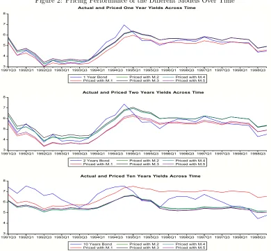
Figure 2 shows the actual and the generated prices for the different maturities. We find that all the pricing models perform better in predicting the shorter maturities than in predicting the longer maturities.18

Table 5: Pricing Performance Results: Relative Mean Square Error, Confusion Rates and Pesaran-Timmermann tests

Maturity

6 Month 1 Year 2 Year 5 Year 10 Year Total Relative Mean Square Error

Model 1 − 0.007756 0.010131 − 0.032819 0.050706

Model 2 − 0.004287 0.009334 − 0.022068 0.035689

Model 3 − 0.005558 0.011438 − 0.021748 0.038743

Model 4 − 0.004379 0.009518 − 0.022269 0.036167

Model 5 − 0.005413 0.011164 − 0.021480 0.038056

Confusion Rates

Model 1 − 0.10

(0.00) (00..1000) − (00..1300) 0.11

Model 2 − 0.10

(0.00) (00..1000) − (00..2700) 0.16

Model 3 − 0.10

(0.00) (00..1700) − (00..3000) 0.19

Model 4 − 0.10

(0.00) (00..1000) − (00..3000) 0.17

Model 5 − 0.10

(0.00) (00..1300) − (00..3000) 0.18 Note: The values are Relative Mean Square Errors of the difference between the generated yields and the actual data for each maturity. In brackets are the (asymptotic) P-value of the success-ratio test statistic.

2) Consider the quantities:

lt=

1 if ∆xt60,

−1 otherwise, and blt=

1 if ∆bxt60,

−1 otherwise,

fort= 1, . . . , T (withT equals to the number of predicted yields). Then, the success ratio, i.e. the fraction of times the direction of changes of the yields are correctly predicted, is given byS= (1/T)PT

t=1I(ltblt>0), whereI(·) is the indicator function. If the model had no power in predicting the changes,{lt}and{blt}would

be independent and the success ratio would be given byS∗_=q

b

q+(1−q)(1−qb), whereq= (1/T) PT

t=1I(lt= 1) andqb= (1/T)

PT

t=1I(blt= 1). Hence, we test whether the difference betweenSandS∗ is statistically significant by using the statistic SR = (S−S∗)/(p

(1/T)ω),whereω=S∗{1−S∗} −q(1−q)(2bq−1) 2₋ b

q(1−qb)(2q−1)

2_{. Under the null hypothesis that actual and predicted changes are independent, SR has a}

standard normal asymptotic distribution.

18_{To evaluate how close are the generated prices to the actual ones, we exclude the two maturities (6}

Figure 2: Pricing Performance of the Different Models Over Time

3 4 5 6 7 8

1991Q31992Q11992Q3 1993Q11993Q3 1994Q11994Q3 1995Q11995Q31996Q1 1996Q31997Q1 1997Q31998Q1 1998Q3 1 Year Bond

Priced with M.1

Priced with M.2 Priced with M.3

Priced with M.4 Priced with M.5

3 4 5 6 7 8

1991Q31992Q11992Q3 1993Q11993Q3 1994Q11994Q3 1995Q11995Q31996Q1 1996Q31997Q1 1997Q31998Q1 1998Q3 2 Years Bond

Priced with M.1

Priced with M.2 Priced with M.3

Priced with M.4 Priced with M.5

3 4 5 6 7 8

1991Q31992Q11992Q3 1993Q11993Q3 1994Q11994Q3 1995Q11995Q31996Q1 1996Q31997Q1 1997Q31998Q1 1998Q3 10 Years Bond

Priced with M.1

Priced with M.2 Priced with M.3

Priced with M.4 Priced with M.5

Actual and Priced One Year Yields Across Time

Actual and Priced Two Years Yields Across Time

Actual and Priced Ten Years Yields Across Time

Pricing Performance of the Different Models Over Time

Figure 2

Table 6 reports the proportion of the times that each model achieves the smallest RMSE over the 30 sample points (1991:3-1998:4). This is calculated on the basis of the individual maturities (1, 2 and 10 years) and the sum of them. We find thatmodel 1 outperforms the alternative switching specifications 60% of the time, while model 5 only outperforms the competing models 5% of the time.

It is very informative to compare the results presented intable 6 with those presented in table 5 (where we look at the average pricing errors). We find for the 10 year rate that the smallest RMSE is achieved by model 5, while when we evaluate the performance in terms of the number of periods with the smallest pricing errors, we find that model 5 only outperforms the competing models 10% of the time and thatmodel 1 achieves the smallest RMSE 63% of the time.

Table 6: Pricing Performance Results: Percentage of the periods where each model outperforms the rival models using the Relative Mean Square (Pricing) Error

Maturity

6 Month 1 Year 2 Year 5 Year 10 Year Total Relative Mean Square Error over Time

Model 1 − 0.57 0.50 − 0.63 0.57

Model 2 − 0.10 0.17 − 0.13 0.13

Model 3 − 0.27 0.27 − 0.07 0.20

Model 4 − 0.03 0.03 − 0.07 0.05

Model 5 − 0.03 0.03 − 0.10 0.05

Note: The reported dates are for the models with lowest Relative Mean Square Errors of the difference between the generated yields and the actual data. The entries are the percentage of time each models achieve the smallest RMSE over the sample size (1991:3-1998:4).

To summarize: the linear model seems to be more successful for pricing bonds over time (i.e. it outperforms the switching models most of the time), while, switching models seem to be more successful on average because they outperform the linear models around the breaks in the data. In fact figure 2 shows that (given that our sample includes two changes in regime: in 1991:3-1995:3 and 1995:4-1998:4) the switching models seem to be useful for pricing 10-year bonds immediately after the break, but their pricing performance deteriorates the further away from the break we evaluate the models.

The poor performance of model 5 (over time), compared with model 1, highlights the fact that attempting to correctly specify the switching model is crucial (especially when the model is used to produce one step ahead prices). This exercise suggests how important it is to carry out a careful model selection of the switching interest rate process, and that failing to do so may give prices that do not represent an improvement over those obtained with models that do not allow for regime switching, even in cases where there are clear breaks in the data.

5

Conclusions

the model is affected by different assumptions about which parameters (drift and diffusion) are specified as regime-dependent. Our approach is based on recursively estimating Markov-switching models for the short-term interest rate and generating bond yields which are then compared with actual yields. We find that the results obtained for the whole sample do not coincide with those obtained using different pricing strategies. These results illustrate that, for the one-factor model analyzed in the paper, Markov-switching specifications provide the best in-sample fit but not necessarily the best ex-ante one step ahead prices.

The main results of the paper can be summarized as follows: (i)for short and medium term maturities, simpler Markov-switching specifications produce better bond prices than those obtained using models where all the parameters are allowed to switch (and models with no regime switching); (ii) the pricing gains of Markov-switching models diminish the further away of the break the bond price is evaluated, to the extent that eventually the no regime switching model beats the Markov-switching model. Nevertheless, some of these findings should not be very surprising, since a similar phenomenon is found in the literature on forecasting with Markov-switching models. These results highlight the importance of paying special attention to the parameterizations of Markov-switching models.

Appendix A. Model 1: The Benchmark CIR Model

The stochastic processes for the two state variables (the stochastic discount factor and the short rate) are given by

Mt+1= exp

"

−rf_t −

_λ

σ

2_x t

2 −

_λ

σ

_√

xtut+1

#

, (A.1)

and

xt+1−xt=κ[θ−xt] +σ

√

xtut+1. (A.2)

These two expressions are used to price bonds in the fundamental pricing equation (9) in the text:

logP_tτ =Et[logMt+1+ logPtτ+1−1] + 1

2V art[logMt+1+ logP

τ−1

t+1 ]. (A.3)

Using the following affine functional form for bond prices

P_tτ = exp [−Aτ−Bτxt], (A.4)

with the boundary condition

P_τ0= 1,

we obtain the expressions Pτ

t and hence P τ−1

t+1 required in (A.3). Substituting them into

(A.3) and using the fact thatEt[Mt+1] = exp[−rtf] = exp[−xt] yield

Aτ+Bτxt= [Aτ−1+Bτ−1κθ] + [1 +Bτ−1(1−κ)]xt−1₂Bτ2−1σ 2_x

t−Bτ−1λxt.

The right side is obtained as follows:

logMt+1+ logPtτ+1−1 = −xt− _σλ 2xt

2 −

λ σ

√

xtut+1−Aτ−1−Bτ−1xt+1

= −[Aτ−1+Bτ−1κθ]−[1 + λσ 2 1

2+Bτ−1(1−κ)]xt

−[ _σλ+Bτ−1σ] √

xtut+1

which has the conditional moments

Et[logMt+1+ logPtτ+1−1] =−[Aτ−1+Bτ−1κθ]−[1 +

_λ

σ

2

1

2+Bτ−1(1−κ)]xt,

and

V art[logMt+1+ logPtτ+1−1] = [ λ

σ+Bτ−1σ] 2_x

t.

Separating the coefficients on the constant and on the terms inxin (A.5) gives us a set of difference equations forAτ andBτ

Bτ = 1 + (1−κ−λ)Bτ−1−1₂Bτ2−1σ2, Aτ =Aτ−1+Bτ−1κθ.

(A.6)

The boundary conditionP_τ0= 1 implies that

A0=B0= 0.

Given values for θ, κ, σ, λ and subject to the above boundary condition we can easily evaluateAτ andBτ in (A.6). The exponential form of (A.4) means that log prices and log

yields are linear functions of the interest rate (factor)

y_tτ=−logP

τ t

τ =

Aτ

τ +

Bτ

τ xt.

Appendix B. The CIR Model with Regime Switching

Assuming that within regimest+1the evolution of the short rate under physical (historical)

measure_Pfollows the process (5) in the text

xt+1−xt=κ(st+1)[θ(st+1)−xt] +σ(st+1)

√

xtut+1, (B.1)

and that, the pricing kernel allowing for changes in regime takes the form

Mt+1(st+1) = exp

"

−rf_t −

_λ(s t+1) σ(st+1)

2_x t

2 −

λ(st+1) σ(st+1)

√

xtut+1

#

, (B.2)

then, (zero-coupon) bond prices in regimest=iare given by

Ptτ(st=i) = exp [−Aτ(i)−Bτ(i)xt], (B.3)

where

Aτ(i) = πii(Aτ−1(i) +Bτ−1(i)κiθi) +πij(Aτ−1(j) +Bτ−1(j)κjθj) i6=j,

Bτ(i) = πii

(1−κi−λi)Bτ−1(i)−

B_τ2₋₁(i)

2 σ

2

i + 1

+πij

(1−κj−λj)Bτ−1(j)− B2

τ−1(j)

2 σ

2

j + 1

with initial conditionsA0(i) = 0 andB0(i) = 0.

Proof: Notice that when the underlying process is subject to regime shifts, the funda-mental bond pricing equation (9) becomes

P_tτ(st=i) = X

j=0,1

πijEtMt+1(st+1)Ptτ+1−1(st+1)|st+1=j (B.4)

= πi0Et

Mt+1(j)Ptτ+1−1(j)|j= 0

+πi1Et

Mt+1(j)Ptτ+1−1(j)|j= 1

.

Then we can calculate the following relationships:

i) Conditional onst= 0 we can write

P_tτ(st= 0) =π00Et

Mt+1(0)Ptτ+1−1(0)

+π01Et

Mt+1(1)Ptτ+1−1(1)

.

ii) Conditional onst= 1 we can write

Ptτ(st= 1) =π10Et

Mt+1(0)Ptτ+1−1(0)

+π11Et

Mt+1(1)Ptτ+1−1(1)

. (B.5)

Notice that under the informational assumptions of Bansal and Zhou (2002)

Et

h

Mt+1(0)Ptτ−+11(0) i

=Et exp

"

−rf_t −

λ0 σ0 2 xt 2 − λ0 σ0 √

xtut+1−Aτ−1(0)−Bτ−1(0)xt+1 #!

and

Et

h

Mt+1(1)P_tτ−₊₁1(1) i

=Et exp

"

−rft −

_λ 1 σ1 2_x t 2 − λ1 σ1 √

xtut+1−Aτ−1(1)−Bτ−1(1)xt+1 #!

,

which allows us to express the pricing equation (B.4) as

exp [−Aτ(0)−Bτ(0)xt] =

π00Et 

exp 

 −

rf_t −

_λ 0 σ0 2 xt 2 − λ0 σ0 √

xtut+1

−Aτ−1(0)−Bτ−1(0)xt+1



 



+π01Et 

exp 



−r_tf−

_λ1 σ1 2 xt 2 − λ1 σ1 √

xtut+1

−Aτ−1(1)−Bτ−1(1)xt+1



 

, (B.6)

and

exp [−Aτ(1)−Bτ(1)xt] =

π10Et 

exp 



−rf_t −

_λ0 σ0 2 xt 2 − λ0 σ0 √

xtut+1

−Aτ−1(0)−Bτ−1(0)xt+1



 



+π11Et 

exp 



−r_tf−

λ1 σ1 2 xt 2 − λ1 σ1 √

xtut+1

−Aτ−1(1)−Bτ−1(1)xt+1



 

To arrive to the final result we notice that

Et exp "

−r_tf−

_λ 0 σ0 2_x t 2 − λ0 σ0 √

xtut+1−Aτ−1(0)−Bτ−1(0)xt+1

#!

=

exp(−rf_t −

λ0 σ0

2

xt

2 −Aτ−1(0))Et

exp −λ0 σ0 √

xtut+1−Bτ−1(0)xt+1

and that Et exp −λ0 σ0 √

xtut+1−Bτ−1(0)xt+1

= exp _λ 0 σ0 2_x t

2 −Bτ−1(0)(xt+κ0[θ0−xt]) +

B2

τ−1(0)

2 σ

2

0xt+Bτ−1(0)λ0xt !

This last result holds since

Etexp

−λ0

σ0

√

xtut+1

= exp( _λ0 σ0 2_x t

2) whereut+1˜N(0,1),

Et(exp [−Bτ−1(0)xt+1]) = exp

−Bτ−1(0)(xt+κ0[θ0−xt]) +

B2

τ−1(0)

2 σ

2 0xt

,

and that the cross term that enters in the variance isBτ−1(0)λ0xt.

Putting all this results together we obtain that

Et

exp

−rft −

λ02

2 xt−λ0 √

xtut+1−Aτ−1(0)−Bτ−1(0)xt+1

=

exp(−rft −Aτ−1(0)−Bτ−1(0)(xt+κ0[θ0−xt]) +

B2

τ−1(0)

2 σ

2

0xt+Bτ−1(0)λ0xt)

Using the log-linear approximation expx≈1 +xas in Bansal and Zhou (2002) and the

fact thatxt=r f

t, we get the following pricing relationships:

i) Conditional on the current regimest= 0,

[−Aτ(0)−Bτ(0)xt] =

π00(−xt−Aτ−1(0)−Bτ−1(0)(xt+κ0[θ0−xt]) +

B2

τ−1(0)

2 σ

2

0xt+Bτ−1(0)λ0xt)

+π01(−xt−Aτ−1(1)−Bτ−1(1)(xt+κ1[θ1−xt]) +

Bτ2−1(1)

2 σ

2

ii) Conditional on the current regimest= 1,

[−Aτ(1)−Bτ(1)xt] =

π10(−xt−Aτ−1(0)−Bτ−1(0)(xt+κ0[θ0−xt]) +

B2_τ−1(0)

2 σ

2

0xt+Bτ−1(0)λ0xt)

+π11(−xt−Aτ−1(1)−Bτ−1(1)(xt+κ1[θ1−xt]) +

B2

τ−1(1)

2 σ

2

1xt+Bτ−1(1)λ1xt).

(B.9)

Finally equating the constant terms and the terms in xt we obtain that

Aτ(0) = π00(Aτ−1(0) +Bτ−1(0)κ0θ0) +π01(Aτ−1(1) +Bτ−1(1)κ1θ1)

Bτ(0) = π00

(1−κ0−λ0)Bτ−1(0)−

B_τ2₋₁(0)

2 σ

2 0+ 1

+π01

(1−κ1−λ1)Bτ−1(1)− B2

τ−1(1)

2 σ

2 1+ 1

Aτ(1) = π10(Aτ−1(0) +Bτ−1(0)κ0θ0+π11(Aτ−1(1) +Bτ−1(1)κ1θ1)

Bτ(1) = π10

(1−κ0−λ0)Bτ−1(0)− B2

τ−1(0)

2 σ

2 0+ 1

+π11

(1−κ1−λ1)Bτ−1(1)− B2

τ−1(1)

2 σ

2 1+ 1

Appendix C. Maximum Likelihood Estimation

The estimates of the regime-swtching models are obtained using procedures which are iden-tical to those described by (Hamilton, 1988, 1989), except that in this case the short term interest rate and the yields of the two maturities observed with error (the six months bill and the 5 years bond) depend on the state of the economy. The density of the data yt

conditional on the statest and the history of the system can be written as

P(yt|st, yt−1, ..., y1 : Θ) =

1 (2π).5_σ

st

√ xt−1

exp(−(σ2stxt−1)

−1

(∆xt−κ(st)[θ(st)−xt−1])2)

× 1

2π|Σst|1/2

exp(−1

2u

0 tΣ

−1

stut),

whereytis a 3×1 vector containing the 3months T-bill,xt,the 6 month T-bill,y2t,and the

5 years bond,y20

t ,where

ut= "

y2

t−

A2(st)

2 +

B2(st)

2 xt y20t −

A20(st)

2 +

B20(st)

2 xt

#

, Σ₀ =

"

σ2

0(6m) σ0(6m,5y) σ0(6m,5y) σ20(5y)

#

,

Σ1 =

"

σ2

1(6m) σ1(6m,5y) σ1(6m,5y) σ1(52 y)

#

, and Aτ(st) and Bτ(st) are generated as in Appendix

The pricing (and estimation) is carried out recursively and the one step ahead prices are computed as Atτ−1(st−1)

2 +

Bt_τ−1(st−1)

2 xt, where Aτt−1 and Bτt−1 are obtained using the

estimates obtained att−1 (since they use information of the long term bonds). For the one step ahead pricing we use the short term interest rates at time t (which are observed and assumed exogenous) to price the bonds at time t. In this way we do not use information about the contemporaneous long yields to price them.

References

Ang, A. and G. Bekaert (2002a): “Regime switches in interest rates,”Journal of Business and Economic Statistics, 20, 163–182.

Ang, A. and G. Bekaert (2002b): “Short rate nonlinearities and regime switches,”Journal of Economic Dynamics and Control, 26, 1243–1274.

Bansal, R. and H. Zhou (2002): “Term structure of interest rates with regime shifts,”Journal of Finance, 57, 1997–2043.

Bossaerts, P. and P. Hillion (1999): “Implementing statistical criteria to select return fore-casting models: What do we learn?” Review of Financial Studies, 12, 405428.

Cox, J. C., J. E. Ingersoll, and S. A. Ross (1985): “A theory of the term structure of interes rates,”Econometrica, 53, 385–407.

Dahlquist, M. and S. F. Gray (2000): “Regime-switching and interest rates in the european monetary system,”Journal of International Economics, 50, 399–419.

Dai, Q. and K. Singleton (2003): “Term structure dynamics in theory and reality,”Review of Financial Studies, 16, 631–678.

Diebold, F. and C. Li (2006): “Forecasting the term structure of government bond yields,”

Journal of Econometrics, 130, 337–364.

Duffee, G. R. (2002): “Term premia and interest rate forecasts in affine models,”Journal of Finance, 57, 405–443.

Evans, M. (2003): “Regime shifts, risk and the term structure,” Economic Journal, 113, 345–389.

Garcia, R. (1998): “Asymptotic null distribution of the likelihood ratio test in markov switching models,”International Economic Review, 39, 763–788.

Garcia, R. and P. Perron (1996): “An analysis of the real interest rate under regime shifts,”

Review of Economics and Statistics, 78, 111–125.

Granger, C., M. King, and H. White (1995): “Comments on testing economic theories and the use of model selection criteria,”Journal of Econometrics, 67, 172187.

Gray, S. F. (1996): “Modeling the conditional distribution of interest rates as a regime-switching process,”Journal of Financial Economics, 42, 27–62.

Hamilton, J. D. (1988): “Rational expectations econometric analysis of changes in regime: An investigation of the term structure of interest rates,”Journal of Economic Dynamics and Control, 12, 385–423.

Hamilton, J. D. (1989): “A new approach to the economic analysis of nonstationary time series and the business cycle,”Econometrica, 57, 357–384.

Hansen, B. E. (1992): “The likelihood ratio test under non-standard conditions: Testing the markov switching model of gnp,”Journal of Applied Econometrics, 7, S61–S82.

Hansen, B. E. (1996): “Erratum: The likelihood ratio test under non-standard conditions: Testing the markov switching model of gnp,”Journal of Applied Econometrics, 11, 195– 198.

Kapetanios, G. (2001): “Model selection in threshold models,” Journal of Time Series Analysis, 22, 733–754.

Kim, C.-J. and J. M. Piger (2002): “Common stochastic trends, common cycles, and asym-metry in economic fluctuations,”Journal of Monetary Economics, 49, 1189–1211.

Landen, C. (2000): “Bond pricing in a hidden markov model of the short rate,” Finance and Stochastics, 4, 371–390.

Leroux, B. (1992): “Maximum-likelihood estimation for hidden markov-models,”Stochastic Processes and their Applications, 40, 127143.

Leroux, B. and M. Puterman (1992): “Maximum penalized likelihood estimation for inde-pendent and markov-deinde-pendent poisson mixtures,”Biometrics, 48, 545558.

Naik, V. and M. H. Lee (1997): “Yield curve dynamics with discrete shifts in economic regimes,”Faculty of Commerce, University of British Columbia, Working Paper.

Nishii, R. (1988): “Maximum likelihood principle and model selection when the true model is unspecified,”Journal of Multivariate Analysis, 27, 392–403.

Pearson, N. and T. Sun (1994): “Exploiting the conditional density in estimating the term structure: An application to the cox, ingersoll, and ross model,”Journal of Finance, 49, 1279–1304.

Pesaran, M. H. and A. Timmermann (1992): “A simple nonparametric test of predictive performance,”Journal of Business and Economic Statistics, 10, 461–465.

Pesaran, M. H. and A. Timmermann (1995): “Predictability of stock returns: Robustness and economic significance,”Journal of Finance, 50, 1201–1228.

Psaradakis, Z. and N. Spagnolo (2003): “On the determination of the number of regimes in markov-switching autoregressive models,”Journal of Time Series Analysis, 24, 237–252.

Psaradakis, Z. and N. Spagnolo (2006): “Joint determination of the state dimension and autoregressive order for models with markov regime switching,”Journal of Time Series Analysis, 27, 753–756.

Sin, C.-Y. and H. White (1996): “Information criteria for selecting possibly misspecified parametric models,”Journal of Econometrics, 71, 207225.

Smith, D. R. (2002): “Markov-switching and stochastic volatility in short-term interest rates,”Journal of Business and Economic Statistics, 20, 183–197.

Sola, M. and J. Driffill (1994): “Testing the term structure of interest rates from a stationary switching regime var,”Journal of Economic Dynamics and Control, 18, 601–628.