Comparison of Two Time Series Decomposition Methods: Least Squares and Buys Ballot Methods

ISSN Online: 2161-7198 ISSN Print: 2161-718X

Comparison of Two Time Series Decomposition

Methods: Least Squares and Buys-Ballot Methods

I. S. Iwueze

1

, E. C. Nwogu

1

, V. U. Nlebedim

1

, J. C. Imoh

2

1_{Department of Statistics, Federal University of Technology, Owerri, Nigeria} 2_{Dept of Maths/Statistics, Imo State Polytechnic, Umuagwo, Nigeria}

Abstract

This paper discusses comparison of two time series decomposition methods: The Least Squares Estimation (LSE) and Buys-Ballot Estimation (BBE) methods. As noted by Iwueze and Nwogu (2014), there exists a research gap for the choice of ap-propriate model for decomposition and detection of presence of seasonal effect in a series model. Estimates of trend parameters and seasonal indices are all that are needed to fill the research gap. However, these estimates are obtainable through the Least Squares Estimation (LSE) and Buys-Ballot Estimation (BBE) methods. Hence, there is need to compare estimates of the two methods and recommend. The com-parison of the two methods is done using the Accuracy Measures (Mean Error (ME)), Mean Square Error (MSE), the Mean Absolute Error (MAE), and the Mean Absolute Percentage Error (MAPE). The results from simulated series show that for the additive model; the summary statistics (ME, MSE and MAE) for the two estima-tion methods and for all the selected trending curves are equal in all the simulaestima-tions both in magnitude and direction. For the multiplicative model, results show that when a series is dominated by trend, the estimates of the parameters by both methods become less precise and differ more widely from each other. However, if conditions for successful transformation (using the logarithmic transform in linearizing the multiplicative model to additive model) are met, both of them give similar results.

Keywords

Decomposition Models, Least Squares Estimates, Buys-Ballot Estimates, Accuracy Measures, Successful Transformation, Trending Curves

1. Introduction

The two major goals of time series analysis are 1) identification of the nature of the phenomenon represented by the sequence of observations and 2) forecasting (predict-How to cite this paper: Iwueze, I.S.,

Nwogu, E.C., Nlebedim, V.U. and Imoh, J.C. (2016) Comparison of Two Time Series Decomposition Methods: Least Squares and Buys-Ballot Methods. Open Journal of Statistics, 6, 1123-1137.

http://dx.doi.org/10.4236/ojs.2016.66091

Received: August 20, 2016 Accepted: December 18, 2016 Published: December 21, 2016

Copyright © 2016 by authors and Scientific Research Publishing Inc. This work is licensed under the Creative Commons Attribution International License (CC BY 4.0).

http://creativecommons.org/licenses/by/4.0/

ing future values of the time series variable). Identification of the pattern and choice of model in time series data is critical to facilitate forecasting. Thus, these two goals of time series analysis require that the pattern of observed time series data is identified and described. Two patterns that may be present are trend and seasonality.

The trend represents a general systematic linear or (most often) nonlinear compo-nent that changes over time and does not repeat or at least does not repeat within the time range captured by data. As long as the trend is monotonous (consistently increas-ing or decreasincreas-ing) the identification of trend component is not very difficult. Trend analysis (methods for estimating the trend parameters) can be done by three important methods; 1) smoothing [1][2][3][4][5] 2) fitting a mathematical function [6][7] and 3) differencing to make the series stationary in the ARIMA methodology [1] [8] [9]. Tests for trend are given in Kendall and Ord [7]. Correlation analysis can also be used to assess trend. If a time series contains a trend, then the values of the autocorrelations will not come to zero except for very large values of the lag [6].

Many time series exhibit a variation which repeats itself in systematic intervals over time and this behaviour is known as seasonal dependency (seasonality). By seasonality, we mean periodic fluctuations. It is formally defined as correlational dependency of order k between each ith element of the series and the (i − k)th element [10] and meas-ured by autocorrelation (a correlation between Xt and Xt k− ); k is usually called the

lag. Seasonality can be visually identified in the series as a pattern that repeats every k elements. The following graphical techniques can be used to detect seasonality: 1) A run sequence plot [11], 2) A seasonal sub-series plot [12], 3) Multiple box plots [11] and 4) the autocorrelation plot [1]. Both the seasonal sub-series plot and the box plot assume that the seasonal periods are known. In most cases, the seasonal periods are easy to find (4 for quarterly data, 12 for monthly data etc). If there is significant seasonality, the autocorrelation plot should show spikes at multiples of lags equal to the period, the seasonal lag (for quarterly data, we would expect to see significant spikes at lag 4, 8, 12, 16, and so on). Davey and Flores [13] proposed a method which adds statistical tests of seasonal indexes for the multiplicative model that helps identify seasonality with greater confidence. Tests for seasonality are also given in Kendall and Ord [7].

In time series analysis, it is assumed that the data consist of a systematic pattern and random noise (error). The systematic pattern consists of the: trend (denoted as Tt), seasonal (denoted as St) and cyclical (denoted as Ct) components. The random noise is the error or irregular component (denoted as It or et), where t stands for the par-ticular point in time. These four classes of time series components may or may not co-exist in real-life data.

multiplica-tive models).

Additive model (when trend, seasonal and cyclical components are additively com-bined):

, 1, 2, ,

t t t t t

X = +T S +C +I t=  n (1.1) Multiplicative model (when trend, seasonal and cyclical components are multiplica-tively combined):

, 1, 2, ,

t t t t t

X = × ×T S C ×I t=  n (1.2) Pseudo-Additive/Mixed Model: (combining the elements of both the additive and multiplicative models):

, 1, 2, ,

t t t t t

X = × ×T S C +I t=  n (1.3) Cyclical variation refers to the long term oscillation or swings about the trend and only long period sets of data will show cyclical fluctuation of any appreciable magni-tude. If short period of time are involved (which is true of all examples of this study), the cyclical component is superimposed into the trend [6] and we obtain a trend-cycle component denoted by Mt. In this case Equations (1.1), (1.2) and (1.3) may be written

as:

, 1, 2, ,

t t t t

X =M +S +I t=  n (1.4) , 1, 2, ,

t t t t

X =M × ×S I t=  n (1.5) and

, 1, 2, ,

t t t t

X =M × +S I t=  n (1.6) where Mt is the trend-cycle component; St is the seasonal component with the property that S_{( )}i−1s+j =Sj, 1, 2,i= ,m, and et is the irregular or random compo-nent. For the additive model (1.1), it is assumed that the irregular/error component et is the Gaussian

(

2

)

1 0,

N σ white noise, while for the multiplicative model (1.2), et is the Gaussian

( )

2

2 1,

N σ white noise. For the additive model (1.1), the assumption is that the sum of the seasonal component over a complete period is zero

0 0 s

j j

S =

 

=

 



∑

,

while for the multiplicative model (1.2), the sum of the seasonal component over a complete period is

0

s j j

S s

=

 

=

 



∑

.

The multiplicative model (1.5) can be linearized to become the additive model (1.4).

* * *

, 1, 2, ,

t t t t

X∗=M +S +e t=  n (1.7)

where * * *

log , log , log , log

t e t t e t t e t t e t

X∗= X M = M S = S e = e . It follows that we can

study the additive model (1.1) and apply the results obtain to the multiplicative model after linearization. The pseudo-additive model is used when the original time series contains very small or zero values. For this reason, this work will discuss only the addi-tive and multiplicaaddi-tive models.

and eliminate Mt for each time period from the actual data either by subtraction for Equation (1.4) or division for Equation (1.5). The de-trended series is obtained as

ˆ

t t

X −M for Equation (1.4) or X_t Mˆ_t for Equation (1.5). In the second step, the seasonal effect is obtained by estimating the average of the de-trended series at each season. The de-trended, de-seasonalized series is obtained as ˆ ˆ

t t t

X −M −S for Equa-tion (1.4) or

(

ˆ ˆ

)

t t t

X M S for Equation (1.5). This gives the residual or irregular com-ponent. Having fitted a model to a time series, one often wants to see if the residuals are purely random. For detailed discussion of residual analysis, see [1][14].

This LSE as describe above is known to be associated with computational difficulties and does not give an insight for choice of models for time series decomposition and detection of presence of seasonal effect in a series.

However, by arranging a series of length n into m rows

(

X( )i−1s+j,i=1, 2,m

)

and s

columns

(

X( )i−1s j+ ,j=1, 2,s

)

, Iwueze et al. [15] showed that the row and column

averages and variances can be used to 1) determine the need for and appropriate trans-formation 2) choose the appropriate model for decomposition, 3) detect the presence of seasonal effect in the series and 4) obtain estimates of the trend parameters and season-al indices of the entire series. In particular, for a seasonseason-al series, the rows represent the periods/years while the columns are the seasons. This two-dimensional arrangement of a series is referred to as Buys-Ballot table, see [16][17].

Using the periodic means

(

X ii., =1, 2,,m

)

, Iwueze and Nwogu [17] constructed

two derived variables, the Chain Base Estimation (CBE) and the Fixed Base Estimation (FBE)-derived variables, on bases of which they derived the estimates of linear trend-cycle parameters. Iwueze and Ohakwe [18] derived the estimates of quadratic trend-cycle parameters from the corresponding CBE and the FBE-derived variables, while Iwueze and Nwogu [19] derived the estimates of the exponential trend-cycle pa-rameters from the corresponding CBE and the FBE-derived variables.

Iwueze and Nwogu [20] have shown that, for seasonal time series data and for all trending curves, the row, column and overall averages and variances of the Buys-Ballot table are 1) functions of the trend parameters and 2) different for the additive and mul-tiplicative models. Therefore, the row, column and overall averages and variances can be used for i) choice of appropriate model, ii) detection of presence of seasonal effect in a series in addition to estimation of trend parameters and seasonal indices. Since esti-mates of the trend parameters and seasonal indices can also be derived from the Least Squares method, there is the need to compare the two decomposition methods.

2. Methodology

The comparison of Least Squares Estimates and Buys-Ballot Estimates in this study is done using measures often referred to in the literature as Forecasting Accuracy Meas-ures. These include the Mean Error (ME), Mean Square Error (MSE), the Mean Abso-lute Error (MAE), and the Mean AbsoAbso-lute Percentage Error (MAPE).

Given the actual values of the parameters θ =i,i 1, 2,L these accuracy measures may be defined in terms of the deviations of the parameter estimates from the corres-ponding actual values used in the simulations. Thus, if ˆ

i

θ

is the estimate of the para-meter θi, then ei= −

θ θ

i ˆi is the error made in estimating θ =i,i 1, 2,L. In terms of

i

e , the accuracy measures adapted from the forecasting Accuracy Measures are

(

)

1 1 Mean Error ME

L i i

e L =

=

∑

_(2.1)

(

)

2

1 1 Mean Square Error MSE

L i i

e L =

=

∑

_(2.2)

(

)

1 1 Mean Absolute Error MAE

L i i

e L =

=

∑

_(2.3)

(

)

1 1 Mean Absolute Percentage Error MAPE 100

L i i i

e

L = θ

 

= _{ }



∑

 (2.4)

In these definitions, the comparison of parameter estimates is done directly using the actual and estimated values of the parameters.

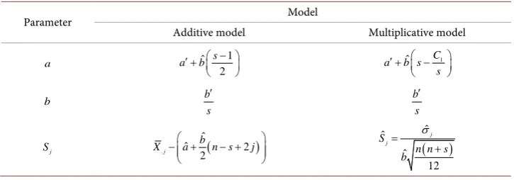
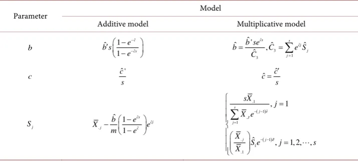
The summary of the estimates of trend parameters and seasonal indices obtained by Iwueze and Nwogu [20] are given in Table 1 for Linear, Table 2 for Quadratic and Ta-ble 3 Exponential trend-cycle component for the additive and multiplicative models.

We note the following for Tables 1-3:

1) a′, b′ and c′ are estimates derived from the regression equations of row av-erages on row number.

2) Additive and Multiplicative models give different estimates.

3) 2

1 2

1 1

ˆ s ˆ _{, .}ˆ s ˆ

j j

j j

C jS C j S

= =

[image:5.595.192.555.568.695.2]

=

∑

=

∑

Table 1. Estimates of parameters of Linear trend-cycle components and seasonal indices.

Parameter Model

Additive model Multiplicative model

a ˆ 1

2

s a′ + b − _

 

1

ˆ C

a b s s   ′ + _ − _   b b s ′ b s ′ j

S . ( )

ˆ

ˆ 2

2

j b

X −_a+ n− +s j _

  ( ) ˆ ˆ ˆ 12 j j S

n n s b

σ =

+

[image:6.595.192.554.89.274.2]

Table 2. Estimates of parameters of quadratic trend-cycle component and seasonal indices.

Parameter Model

Additive model Multiplicative model

a ˆ 1 ˆ ( 1 2)( 1) ˆ

2 6

s s

s

a′ +_ − _b−  − − c

  2 1 2 1 ˆ ˆ ˆ ˆ

ˆ C ˆ 2 C

a b s c s C

s s

   

′ + _ − _− _ − + _

   

b _bˆ bˆ _{c sˆ}( ₁)

s

′

= + −

(

2

)

1

1 2

b c s C s ′ + − 

c

ˆ 2

c c

s

′

= ˆ 2

c c s ′ = j

S Sˆj=X.j−dj Sˆj=X.j dj

j d

( ) ( )( )

( )

(

)

2

ˆ ˆ 2

ˆ

2 6

ˆ _{ˆ ˆ}

c n s n s b

a n s

b c n s j cj

− −

+ − +

+ + − +

( ) ( )( )

( )

(

)

2

ˆ ˆ 2

ˆ

2 6

ˆ _{ˆ ˆ}

c n s n s b

a n s

b c n s j cj

− −

+ − +

+ + − +

[image:6.595.194.552.320.481.2]

Source: Iwueze and Nwogu [20].

Table 3. Estimates of parameters of exponential trend-cycle component and seasonal indices.

Parameter Model

Additive model Multiplicative model

b ˆ ˆ 1 ˆ 1 c cs e b s e − − −   ′ _{ −} _ ˆ ˆ 3 1 3 ˆ '

ˆ _,ˆ ˆ

ˆ cs s cj j j b se

b C e S

C =

= =

∑

c cˆ '

s ˆ ˆ c c s ′ = j S ˆ ˆ . ˆ ˆ 1 1 cs cj j c b e X e m e −   −  ₋    ( ) ( ) .1 ˆ 1 . 1

. 1? 1 .1

, 1

ˆ _{, 1, 2, ,}

s j e J j

j j e

sX j X e

X

S e j s

X − − = − −  ₌       _{  =}     

∑



Source: Iwueze and Nwogu [20].

3. Simulation Examples

This Section presents some simulations examples used to compare the estimates of the parameters of the selected trend curves and seasonal indices using Buys-Ballot method with those based on the conventional Least Squares Estimation method. For the linear trend-cycle, the simulated examples consist of 106 series of 120 observations each si-mulated from Xt=

(

a bt+

)

+ +St et with a=1, 0.02, 0.2b= and 2.0 and

(

0, 1.0

)

t

e ∼N

σ

= for the additive model, Xt=

(

a bt+

)

∗ ∗St et, with 1, 0.02, 0.2, 2.0

a= b= and et∼N

(

1,

σ

=0.02

)

for the multiplicative model. These values of a, b and c were arbitrarily chosen for simulation purposes. The values of

, 1, 2, ,12

j

S j=  for the simulated additive and the multiplicative models are given in Table 4.

[image:7.595.194.553.194.379.2]

devia-tions are computed from the residuals from the fitted models. The deviadevia-tions of these estimates from the parameters used in the simulations are given in Appendix A for the Additive model and Appendix B for the Multiplicative model, while the summary sta-tistics for 20 simulations only are given in Table 5 for the Additive model and Tables 6-8 for the Multiplicative model.

Table 4. Seasonal

( )

Sj indices used in the simulation of series from additive and multiplicative

models.

j Sj

Additive Multiplicative

1 −0.89 0.91

2 −1.22 0.88

3 0.10 1.00

4 −0.15 0.98

5 −0.09 0.98

6 1.16 1.12

7 2.34 1.26

8 1.95 1.20

9 0.64 1.05

10 −0.73 0.92

11 −2.14 0.80

12 −0.97 0.90

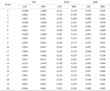
Table 5. Summary statistics for additive model (a = 1 and b = 2).

Series ME MAE MSE

LSE BBE LSE BBE LSE BBE

1 −0.009 −0.009 0.221 0.219 0.074 0.076

2 0.000 0.001 0.156 0.160 0.038 0.041

3 0.003 0.002 0.226 0.228 0.080 0.085

4 −0.003 −0.002 0.213 0.221 0.074 0.078

5 0.002 0.004 0.157 0.159 0.062 0.065

6 0.016 0.017 0.200 0.199 0.071 0.069

7 −0.003 −0.002 0.207 0.214 0.073 0.078

8 0.026 0.027 0.192 0.191 0.072 0.069

9 0.000 0.003 0.180 0.173 0.076 0.075

10 0.024 0.025 0.252 0.256 0.097 0.101

11 0.004 0.004 0.167 0.170 0.048 0.049

12 0.000 −0.002 0.224 0.235 0.131 0.128

13 0.015 0.015 0.220 0.226 0.077 0.078

14 −0.011 −0.010 0.230 0.232 0.093 0.094

15 0.019 0.020 0.215 0.226 0.083 0.092

16 0.010 0.011 0.167 0.172 0.057 0.060

17 0.003 0.004 0.143 0.152 0.041 0.044

18 0.015 0.015 0.274 0.275 0.146 0.148

19 0.002 0.003 0.203 0.203 0.070 0.067

[image:7.595.193.553.411.708.2]

[image:8.595.198.552.88.381.2]

Table 6. Summary statistics for multiplicative model (a = 1 and b = 0.02).

S/N ME MAE MAPE MSE RSME

LSE BBE LSE BBE LSE BBE LSE BBE LSE BBE

1 −0.001 −0.001 0.005 0.012 0.840 2.834 0.000 0.000 0.006 0.016

2 0.000 0.000 0.003 0.013 0.470 3.271 0.000 0.000 0.004 0.018

3 0.000 0.000 0.005 0.014 0.799 3.368 0.000 0.000 0.006 0.018

4 0.000 −0.001 0.004 0.015 0.798 4.924 0.000 0.001 0.006 0.023

5 0.000 0.000 0.003 0.011 0.578 2.873 0.000 0.000 0.005 0.014

6 0.001 0.000 0.004 0.014 0.766 4.834 0.000 0.000 0.006 0.021

7 0.000 −0.001 0.004 0.013 0.773 4.223 0.000 0.000 0.006 0.017

8 0.001 0.000 0.004 0.012 0.883 3.054 0.000 0.000 0.006 0.016

9 0.000 0.000 0.004 0.010 0.713 2.069 0.000 0.000 0.005 0.014

10 0.001 0.000 0.006 0.013 1.055 4.062 0.000 0.000 0.007 0.017

11 0.000 −0.001 0.004 0.018 0.554 6.065 0.000 0.001 0.005 0.023

12 0.000 −0.001 0.005 0.012 1.065 3.591 0.000 0.000 0.008 0.019

13 0.000 0.000 0.004 0.014 0.837 3.310 0.000 0.000 0.006 0.017

14 0.000 −0.001 0.005 0.010 0.989 2.517 0.000 0.000 0.006 0.015

15 0.001 0.000 0.004 0.009 0.893 2.073 0.000 0.000 0.006 0.013

16 0.000 0.000 0.003 0.014 0.577 3.555 0.000 0.000 0.005 0.018

17 0.000 −0.001 0.003 0.015 0.442 4.974 0.000 0.001 0.004 0.023

18 0.000 0.000 0.006 0.008 1.215 1.468 0.000 0.000 0.008 0.012

19 0.000 0.000 0.004 0.013 0.743 3.077 0.000 0.000 0.006 0.018

20 0.000 −0.001 0.005 0.018 0.809 4.686 0.000 0.001 0.000 0.024

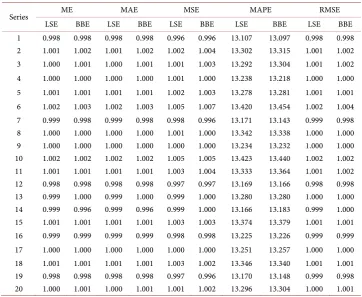
Table 7. Summary statistics for multiplicative model (a = 1 and b = 0.2).

Series ME MAE MSE MAPE RMSE

LSE BBE LSE BBE LSE BBE LSE BBE LSE BBE

1 0.998 0.998 0.998 0.998 0.996 0.996 13.107 13.097 0.998 0.998

2 1.001 1.002 1.001 1.002 1.002 1.004 13.302 13.315 1.001 1.002

3 1.000 1.001 1.000 1.001 1.001 1.003 13.292 13.304 1.001 1.002

4 1.000 1.000 1.000 1.000 1.001 1.000 13.238 13.218 1.000 1.000

5 1.001 1.001 1.001 1.001 1.002 1.003 13.278 13.281 1.001 1.001

6 1.002 1.003 1.002 1.003 1.005 1.007 13.420 13.454 1.002 1.004

7 0.999 0.998 0.999 0.998 0.998 0.996 13.171 13.143 0.999 0.998

8 1.000 1.000 1.000 1.000 1.001 1.000 13.342 13.338 1.000 1.000

9 1.000 1.000 1.000 1.000 1.000 1.000 13.234 13.232 1.000 1.000

10 1.002 1.002 1.002 1.002 1.005 1.005 13.423 13.440 1.002 1.002

11 1.001 1.001 1.001 1.001 1.003 1.004 13.333 13.364 1.001 1.002

12 0.998 0.998 0.998 0.998 0.997 0.997 13.169 13.166 0.998 0.998

13 0.999 1.000 0.999 1.000 0.999 1.000 13.280 13.280 1.000 1.000

14 0.999 0.996 0.999 0.996 0.999 1.000 13.166 13.183 0.999 1.000

15 1.001 1.001 1.001 1.001 1.003 1.003 13.374 13.379 1.001 1.001

16 0.999 0.999 0.999 0.999 0.998 0.998 13.225 13.226 0.999 0.999

17 1.000 1.000 1.000 1.000 1.000 1.000 13.251 13.257 1.000 1.000

18 1.001 1.001 1.001 1.001 1.003 1.002 13.346 13.340 1.001 1.001

19 0.998 0.998 0.998 0.998 0.997 0.996 13.170 13.148 0.999 0.998

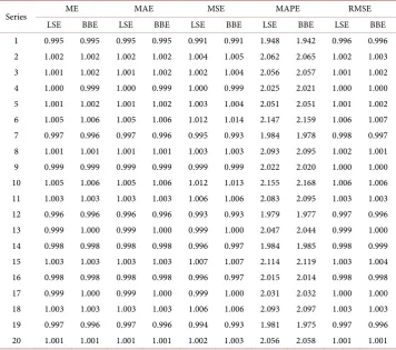
[image:8.595.191.554.410.707.2]

[image:9.595.196.553.89.404.2]

Table 8. Summary statistics for multiplicative model (a = 1 and b = 2.0).

Series ME MAE MSE MAPE RMSE

LSE BBE LSE BBE LSE BBE LSE BBE LSE BBE

1 0.995 0.995 0.995 0.995 0.991 0.991 1.948 1.942 0.996 0.996

2 1.002 1.002 1.002 1.002 1.004 1.005 2.062 2.065 1.002 1.003

3 1.001 1.002 1.001 1.002 1.002 1.004 2.056 2.057 1.001 1.002

4 1.000 0.999 1.000 0.999 1.000 0.999 2.025 2.021 1.000 1.000

5 1.001 1.002 1.001 1.002 1.003 1.004 2.051 2.051 1.001 1.002

6 1.005 1.006 1.005 1.006 1.012 1.014 2.147 2.159 1.006 1.007

7 0.997 0.996 0.997 0.996 0.995 0.993 1.984 1.978 0.998 0.997

8 1.001 1.001 1.001 1.001 1.003 1.003 2.093 2.095 1.002 1.001

9 0.999 0.999 0.999 0.999 0.999 0.999 2.022 2.020 1.000 1.000

10 1.005 1.006 1.005 1.006 1.012 1.013 2.155 2.168 1.006 1.006

11 1.003 1.003 1.003 1.003 1.006 1.006 2.083 2.095 1.003 1.003

12 0.996 0.996 0.996 0.996 0.993 0.993 1.979 1.977 0.997 0.996

13 0.999 1.000 0.999 1.000 0.999 1.000 2.047 2.044 0.999 1.000

14 0.998 0.998 0.998 0.998 0.996 0.997 1.984 1.985 0.998 0.999

15 1.003 1.003 1.003 1.003 1.007 1.007 2.114 2.119 1.003 1.004

16 0.998 0.998 0.998 0.998 0.996 0.997 2.015 2.014 0.998 0.998

17 0.999 1.000 0.999 1.000 0.999 1.000 2.031 2.032 1.000 1.000

18 1.003 1.003 1.003 1.003 1.006 1.006 2.093 2.097 1.003 1.003

19 0.997 0.996 0.997 0.996 0.994 0.993 1.981 1.975 0.997 0.996

20 1.001 1.001 1.001 1.001 1.002 1.003 2.056 2.058 1.001 1.001

For the additive model the results are the same for the selected values of the slope parameter

(

b=0.02, 0.2 and 2.0

)

. Therefore, the summary statistics for b = 2 only is shown in Table 5. As Table 5 shows, the summary statistics (ME, MSE and MAE) for the two estimation methods (LSE and BBE) are equal both in magnitude and direction all the simulations. This indicates that the two methods are equally effective in estimat-ing the trend parameters and seasonal indices when the model for decomposition is ad-ditive.

For the multiplicative model, Table 6 shows that for b = 0.02, the values of the sum-mary statistics (ME, RMSE, MSE, MAE and MAPE) are equal in almost all the simula-tions as in the additive model. However, for values of b = 0.2 and 2.0, Table 7 and Ta-ble 8 show that the values of the summary statistics (ME, RMSE, MSE, MAE and MAPE) are unequal in most all the simulations and the difference increased as the val-ue of b increased from 0.2 to 2.0. In other words, when a series is dominated by trend, not only do the estimates of the parameters by both methods become less precise; esti-mates of the parameters from the two methods differ more widely from each other.

from the two methods and the actual values when b = 0.2 and 2.0 may be attributable to the violation of the condition for successful transformation (linearization in this case). For b = 0.2 and a = 1, b a=0.2 and for b = 2.0 and a = 1, b a=2.0.

For the Quadratic trend-cycle component, the empirical examples also consist of 106 series of 120 observations each simulated from

(

2

)

t t t

X = a+ +bt ct +S +e , with

1, 2.0, 3.0

a= b= c= and et ∼N

(

0,

σ

=1.0

)

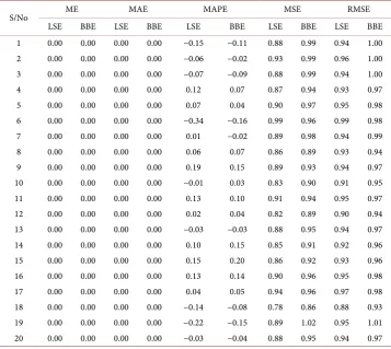
and Sj given in Table 4 for the

addi-tive model only. However, for want of space, the summary statistics for 20 simulations only are given in Table 9. As Table 9 shows, the summary statistics (ME, MSE and MAE) for the two estimation methods (LSE and BBE) are equal in almost all the simu-lations. This indicates that the two methods are equally effective in estimating the trend parameters and seasonal indices when the model for decomposition is additive.

For the Exponential trend-cycle component, the empirical examples also consist of 106 series of 120 observations each simulated from

( )

ct

t t t

X = be +S +e with b=10 and

c

=

0.02

and et N

(

0,

σ

=1.0

)

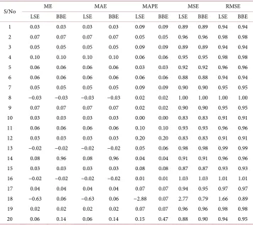
and Sj given in Table 4 for the additive

[image:10.595.194.552.388.707.2]

model only. The summary statistics for 20 simulations given in Table 10 shows that the summary statistics (ME, MSE and MAE) for the two estimation methods (LSE and BBE) are equal in almost all the simulations. This indicates that the two methods are equally effective in estimating the trend parameters and seasonal indices when the model for decomposition is additive.

Table 9. Summary statistics for additive quadratic model (a = 1, b = 2 and c = 3).

S/No ME MAE MAPE MSE RMSE

LSE BBE LSE BBE LSE BBE LSE BBE LSE BBE

1 0.00 0.00 0.00 0.00 −0.15 −0.11 0.88 0.99 0.94 1.00

2 0.00 0.00 0.00 0.00 −0.06 −0.02 0.93 0.99 0.96 1.00

3 0.00 0.00 0.00 0.00 −0.07 −0.09 0.88 0.99 0.94 1.00

4 0.00 0.00 0.00 0.00 0.12 0.07 0.87 0.94 0.93 0.97

5 0.00 0.00 0.00 0.00 0.07 0.04 0.90 0.97 0.95 0.98

6 0.00 0.00 0.00 0.00 −0.34 −0.16 0.99 0.96 0.99 0.98

7 0.00 0.00 0.00 0.00 0.01 −0.02 0.89 0.98 0.94 0.99

8 0.00 0.00 0.00 0.00 0.06 0.07 0.86 0.89 0.93 0.94

9 0.00 0.00 0.00 0.00 0.19 0.15 0.89 0.93 0.94 0.97

10 0.00 0.00 0.00 0.00 −0.01 0.03 0.83 0.90 0.91 0.95

11 0.00 0.00 0.00 0.00 0.13 0.10 0.91 0.94 0.95 0.97

12 0.00 0.00 0.00 0.00 0.02 0.04 0.82 0.89 0.90 0.94

13 0.00 0.00 0.00 0.00 −0.03 −0.03 0.88 0.95 0.94 0.97

14 0.00 0.00 0.00 0.00 0.10 0.15 0.85 0.91 0.92 0.96

15 0.00 0.00 0.00 0.00 0.15 0.20 0.86 0.92 0.93 0.96

16 0.00 0.00 0.00 0.00 0.13 0.14 0.90 0.96 0.95 0.98

17 0.00 0.00 0.00 0.00 0.04 0.05 0.94 0.96 0.97 0.98

18 0.00 0.00 0.00 0.00 −0.14 −0.08 0.78 0.86 0.88 0.93

19 0.00 0.00 0.00 0.00 −0.22 −0.15 0.89 1.02 0.95 1.01

[image:11.595.196.553.88.404.2]

Table 10. Summary statistics for additive exponential model (b = 10 and c = 0.02).

S/No ME MAE MAPE MSE RMSE

LSE BBE LSE BBE LSE BBE LSE BBE LSE BBE

1 0.03 0.03 0.03 0.03 0.09 0.09 0.89 0.89 0.94 0.94

2 0.07 0.07 0.07 0.07 0.05 0.05 0.96 0.96 0.98 0.98

3 0.05 0.05 0.05 0.05 0.09 0.09 0.89 0.89 0.94 0.94

4 0.10 0.10 0.10 0.10 0.06 0.06 0.95 0.95 0.98 0.98

5 0.06 0.06 0.06 0.06 0.03 0.03 0.92 0.92 0.96 0.96

6 0.06 0.06 0.06 0.06 0.06 0.06 0.88 0.88 0.94 0.94

7 0.05 0.05 0.05 0.05 0.09 0.09 0.90 0.90 0.95 0.95

8 −0.03 −0.03 −0.03 −0.03 0.02 0.02 1.00 1.00 1.00 1.00

9 0.07 0.07 0.07 0.07 0.02 0.02 0.90 0.90 0.95 0.95

10 0.03 0.03 0.03 0.03 0.00 0.00 0.83 0.83 0.91 0.91

11 0.06 0.06 0.06 0.06 0.10 0.10 0.93 0.93 0.96 0.96

12 0.03 0.03 0.03 0.03 0.20 0.20 0.83 0.83 0.91 0.91

13 −0.02 −0.02 −0.02 −0.02 0.05 0.06 0.98 0.98 0.99 0.99

14 0.08 0.96 0.08 0.96 0.04 0.04 0.91 0.91 0.96 0.96

15 0.03 0.03 0.03 0.03 0.08 0.08 0.87 0.87 0.93 0.93

16 −0.02 −0.02 −0.02 −0.02 0.01 0.01 1.03 1.03 1.01 1.01

17 0.04 0.04 0.04 0.04 0.07 0.07 0.94 0.95 0.97 0.97

18 −0.63 0.06 −0.63 0.06 −2.88 0.07 2.77 0.79 1.66 0.89

19 0.02 0.02 0.02 0.02 0.07 0.07 0.96 0.96 0.98 0.98

20 0.06 0.14 0.06 0.14 0.15 0.47 0.88 0.90 0.94 0.95

4. Summary, Recommendation and Conclusion

This study has compared the estimates of trend parameters and seasonal indices from the Buys Ballot method with the results from the Least Squares Estimation (LSE) method for the linear, quadratic and exponential trending curves. The rationale for this study is to assess the performance of the Buys Ballot Estimation (BBE) method in rela-tion to the Least Squares Estimarela-tion (LSE) method.

The comparison of Least Squares Estimates and Buys-Ballot Estimates in this study is done using Accuracy Measures (the Mean Error (ME), Mean Square Error (MSE), the Mean Absolute Error (MAE), and the Mean Absolute Percentage Error (MAPE)). These Accuracy Measures are defined, for each estimation procedure, in terms of the deviations of the parameter estimates (using simulated series) from the corresponding actual values used in the simulations.

The results of the analyses show that, for the additive model the summary statistics (ME, MSE and MAE) are equal both in magnitude and direction all the simulations for the two estimation methods (LSE and BBE) and all the selected trending curves. This indicates that the two estimation methods are equally effective in estimating the trend parameters and seasonal indices when the model for decomposition is additive.

MSE, MAE and MAPE) are equal in all the simulations as in the additive model. How-ever, as the value of b increased from 0.02 to 2.0 the results show that the values of the summary statistics (ME, RMSE, MSE, MAE and MAPE) are unequal in all the simula-tions and the difference increases with an increase in b. In other words, when a series is dominated by the trend, the estimates of the parameters by both methods become less precise and differ more widely from each other. This has been attributed to the viola-tion of the condiviola-tion for successful transformaviola-tion (linearizaviola-tion in this case). It could be recalled that logarithm transformation of the multiplicative model to the additive model can preserve the linearity of a linear trend only if the trend parameters (a and b) satisfy the condition; −0.01≤b a≤0.06 [21]).

Therefore, when the model is additive, the estimates of trend parameters and sea-sonal indices are the same for both estimation procedures. However, because of the in-sight it gives into choice of model and detection of presence of seasonal effect, the BBE is recommended.

References

[1] Box, G.E.P., Jenkins, G.M. and Reinsel, G.C. (1994) Time Series Analysis; Forecasting and Control. 3rd Edition, Prentice Hall, Englewood Cliff, New Jersey.

[2] Velleman, P.F. and Hoaglin, D.C. (1981) Applications, Basics and Computing of Explora-tory Data Analysis Duxbury Press, Boston.

[3] Makridakis, S.G., Wheelwright, S.C. and McGee, V.E. (1983) Forecasting: Methods and Applications. 2nd Edition, Wiley, New York.

[4] Gardner Jr., E.S. (1985) Exponential Smoothing: The State of the Art. Journal of Forecast-ing, 4, 1-28.https://doi.org/10.1002/for.3980040103

[5] Montgomery, D.C., Johnson, L.A. and Gardiner, J.S. (1990) Forecasting and Time Series Analysis. 2nd Edition, McGraw-Hill, New York.

[6] Chatfield, C. (2004) The Analysis of Time Series: An Introduction, Chapman and Hall. CRC Press, Boca Raton.

[7] Kendall, M. and Ord, J.K. (1990) Time Series. 3rd Edition, Griffin, London.

[8] Pankratz, A. (1983) Forecasting with Univariate Box-Jenkins Models: Concepts and Cases. Wiley, New York.https://doi.org/10.1002/9780470316566

[9] Wei, W.W. (1989) Time Series Analysis: Univariate and Multivariate Methods. Addi-son-Wesley, New York.

[10] Kendall, M.G. and Stuart, A. (1976) The Advanced Theory of Statistics. Volume 3: Design and Analysis, and Time-Series. Charles Griffin & Co. Ltd., London & High Wycombe. [11] Chambers, J.M., Cleveland, W.S., Kleiner, B. and Tukey, P.A. (1983) Graphical Methods for

Data Analysis. Wadsworth, Bellmont.

[12] Cleveland, W.S. (1993) Visualizing Data. AT&T, Murray Hill.

[13] Davey, A.M. and Flores, B.E. (1993) Identification of Seasonality in Time Series: A Note,

Mathematical and Computer Modelling, 18, 73-81.

https://doi.org/10.1016/0895-7177(93)90126-J

[14] Ljung, G.M. and Box, G.E.P. (1978) On a Measure of Lack of Fit in Time Series Models,

Biometrika, 65, 297-304. https://doi.org/10.1093/biomet/65.2.297

Ta-ble in Time Series Analysis. Applied Mathematics, 2, 633-645.

https://doi.org/10.4236/am.2011.25084

[16] Wold, H. (1938) A Study in the Analysis of Stationary Time Series. 2nd Edition, Almqris-tand Witsett, Stockhol.

[17] Iwueze, I.S and Nwogu, E.C. (2004) Buys-Ballot Estimates for Time Series Decomposition,

Global Journal of Mathematics, 3, 83-98. https://doi.org/10.4314/gjmas.v3i2.21356

[18] Iwueze, I.S. and Ohakwe, J. (2004) Buys-Ballot Estimates When Stochastic Trend Is Qua-dratic. Journal of the Nigerian Association of Mathematical Physics, 8, 311-318.

[19] Iwueze, I.S and Nwogu, E.C. (2005) Buys-Ballot Estimates for Exponential And S-Shaped Curves, for Time Series. Journal of the Nigerian Association of Mathematical Physics, 9, 357-366.

[20] Iwueze, I.S and Nwogu, E.C. (2014) Framework for Choice of Models and Detection of Seasonal Effect in Time Series. Far-East Journal of Theoretical Statistics, 48, 45-66.

[21] Iwueze, I.S. and Akpanta, A.C. (2007) Effect of the Logarithmic Transformation on the Trend-Cycle Component. Journal of Applied Sciences, 7, 2414-2422.

Appendix A

Deviations of the Buys-Ballot and Least Squares estimates of the linear trend parame-ters and seasonal indices from the Parameter values (for Additive model with a = 1and b= 2.0).

S/no Parameter Parameter Value X1 X2 X3

LSE Error BB Error LSE Error BB Error LSE Error BB Error

1 θ =1 a 1.00 1.207 −0.207 1.198 −0.198 1.031 −0.031 1.016 −0.016 1.004 −0.004 1.018 −0.018

2 θ =2 b 2.00 1.997 0.003 1.997 0.003 1.999 0.001 2.000 0.000 2.000 0.000 2.000 0.000

3 θ =3 S1 −0.89 −0.633 −0.257 −0.627 −0.263 −0.728 −0.162 −0.710 −0.180 −1.026 0.136 −1.002 0.112

4 θ =4 S2 −1.22 −1.503 0.283 −1.523 0.303 −1.029 −0.191 −1.010 −0.210 −0.886 −0.334 −0.901 −0.319

5 θ =5 S3 0.10 0.224 −0.124 0.180 −0.080 −0.268 0.368 −0.309 0.409 −0.027 0.127 −0.001 0.101

6 θ =6 S4 −0.15 −0.078 −0.072 −0.117 −0.033 −0.075 −0.075 −0.109 −0.041 −0.523 0.373 −0.501 0.351

7 θ =7 S5 −0.09 −0.455 0.365 −0.413 0.323 −0.021 −0.069 −0.009 −0.081 −0.554 0.464 −0.600 0.510

8 θ =8 S6 1.16 1.283 −0.123 1.290 −0.130 1.457 −0.297 1.492 −0.332 1.219 −0.059 1.200 −0.040

9 θ =9 S7 2.34 1.782 0.558 1.793 0.547 2.208 0.132 2.192 0.148 2.536 −0.196 2.500 −0.160

10 θ =10 S8 1.95 2.376 −0.426 2.397 −0.447 1.804 0.146 1.792 0.158 1.486 0.464 1.500 0.450

11 θ =11 S9 0.64 0.865 −0.225 0.900 −0.260 0.763 −0.123 0.792 −0.152 1.057 −0.417 1.101 −0.461

12 θ =12 S10 −0.73 −0.432 −0.298 −0.397 −0.333 −1.005 0.275 −1.007 0.277 −0.390 −0.340 −0.399 −0.331

13 θ =13 S11 −2.14 −2.566 0.426 −2.593 0.453 −2.438 0.298 −2.407 0.267 −2.355 0.215 −2.399 0.259

14 θ =14 S12 −0.97 −0.863 −0.107 −0.890 −0.080 −0.668 −0.302 −0.707 −0.263 −0.537 −0.433 −0.498 −0.472

15 θ15=µ 0.00 0.000 0.000 0.002 −0.002 0.000 0.000 0.000 0.000 0.000 0.000 −0.001 0.001

16 θ16=σ 1.00 0.944 0.056 0.944 0.056 0.974 0.026 0.974 0.026 0.945 0.055 0.945 0.055

ME −0.009 −0.009 0.000 0.001 0.003 0.002

MAE 0.221 0.219 0.156 0.160 0.226 0.228

MSE 0.074 0.076 0.038 0.041 0.080 0.085

Appendix B

Deviations of the Buys-Ballot and Least Squares estimates of the linear trend parame-ters and seasonal indices from the Parameter values (Multiplicative Model and b = 0.02).

S/no Parameter Parameter Value U1 U2 U3

LSE Error BB Error LSE Error BB Error LSE Error BB Error

1 θ =1 a 1.00 1.011 −0.011 1.009 −0.009 0.999 0.001 0.997 0.003 0.999 0.001 0.998 0.002

2 θ =2 b 0.02 0.020 0.000 0.020 0.000 0.020 0.000 0.020 0.000 0.020 0.000 0.020 0.000

3 θ =3 S1 0.91 0.914 −0.004 0.938 −0.028 0.913 −0.003 0.910 0.000 0.908 0.002 0.914 −0.004

4 θ =4 S2 0.88 0.875 0.005 0.851 0.029 0.883 −0.003 0.888 −0.008 0.886 −0.006 0.901 −0.021

5 θ =5 S3 1.00 1.002 −0.002 0.995 0.005 0.993 0.007 0.992 0.008 0.998 0.002 0.966 0.034

6 θ =6 S4 0.98 0.981 −0.001 1.014 −0.034 0.982 −0.002 0.985 −0.005 0.973 0.007 0.973 0.007

7 θ =7 S5 0.98 0.973 0.007 0.968 0.012 0.981 −0.001 0.962 0.018 0.971 0.009 0.966 0.014

8 θ =8 S6 1.12 1.123 −0.003 1.136 −0.016 1.127 −0.007 1.124 −0.004 1.121 −0.001 1.136 −0.016

9 θ =9 S7 1.26 1.246 0.014 1.232 0.028 1.257 0.003 1.242 0.018 1.265 −0.005 1.295 −0.035

Continued

11 θ =11 S9 1.05 1.055 −0.005 1.056 −0.006 1.053 −0.003 1.073 −0.023 1.059 −0.009 1.070 −0.020

12 θ =12 S10 0.92 0.926 −0.006 0.914 0.006 0.915 0.005 0.889 0.031 0.926 −0.006 0.901 0.019

13 θ =13 S11 0.80 0.793 0.007 0.799 0.001 0.795 0.005 0.777 0.023 0.797 0.003 0.773 0.027

14 θ =14 S12 0.90 0.902 −0.002 0.903 −0.003 0.905 −0.005 0.914 −0.014 0.908 −0.008 0.911 −0.011

15 θ15=µ 1.00 1.000 0.000 1.000 0.000 1.000 0.000 1.001 −0.001 1.000 0.000 1.002 −0.002

16 θ16=σ 0.02 0.019 0.001 0.025 −0.005 0.020 0.000 0.026 −0.006 0.019 0.001 0.026 −0.006

ME 1.000 −0.001 1.000 −0.001 1.000 0.000 1.001 0.000 1.000 0.000 1.002 0.000

MAE 1.000 0.005 1.000 0.012 1.000 0.003 1.001 0.013 1.000 0.005 1.002 0.014

MAPE 51.441 0.840 51.418 2.834 51.528 0.470 51.639 3.271 51.529 0.799 51.657 3.368

MSE 1.000 0.000 1.000 0.000 1.001 0.000 1.004 0.000 1.001 0.000 1.004 0.000

RMSE 1.000 0.006 1.000 0.016 1.000 0.004 1.002 0.018 1.000 0.006 1.002 0.018

Submit or recommend next manuscript to SCIRP and we will provide best service for you:

Accepting pre-submission inquiries through Email, Facebook, LinkedIn, Twitter, etc. A wide selection of journals (inclusive of 9 subjects, more than 200 journals)

Providing 24-hour high-quality service User-friendly online submission system Fair and swift peer-review system

Efficient typesetting and proofreading procedure

Display of the result of downloads and visits, as well as the number of cited articles Maximum dissemination of your research work

Submit your manuscript at: http://papersubmission.scirp.org/