Inter generational effect of parental time and its policy implications

Munich Personal RePEc Archive

Inter-generational effect of parental time

and its policy implications

Zhu, Guozhong and Vuralz, Gulfer

Guanghua School of Management, Peking University, Department of

International Trade, Bogazici University

May 2012

Online at

https://mpra.ub.uni-muenchen.de/40670/

Inter-generational Effect of Parental Time and

Its Policy Implications

∗

Guozhong Zhu

and Gulfer Vural

Abstract

Why do parents with more human capital spend more time

teach-ing and takteach-ing care of their children, in spite of the higher opportunity

cost? How does this affect inter-generational mobility and wage

in-equality? Does this have any implications on the policy that provides

public schooling through income taxation? We develop and estimate a

theoretical model to answer these questions, in the light that parental

time investment is a powerful means of transmitting human capital

inter-generationally.

JEL Classification: E20, R20, R30.

Keywords: Human capital production, Parental time investment, Wage

inequality, Earnings persistence, Public schooling.

∗_{For helpful critiques and suggestions, We thank Marina Azzimonti, Sandra Black,}

Russell Cooper, Dean Corbae, and seminar participants at the University of Texas at

Austin, Renmin University and Shanghai University of Finance and Economics.

1

Introduction

Empirical studies reveal that parental time with children is strongly

posi-tively correlated with parents’ human capital, proxied by either wage rate or

educational attainment. Using the 2003-2006 waves of the American Time

Use Survey, Guryan et al. (2008) document a positive wage/education

gradi-ent in child care time which holds true for differgradi-ent categories of child care,

including basic, educational, recreational and travel-related child care.

Sim-ilar patterns have been documented in many earlier studies, although in a

less comprehensive way. Positive wage gradient of parental time is found

in Hill and Stafford (1974), Kimmel and Connelly (2007) and others; while

positive education gradient is seen in Leibowitz (1974b), Leibowitz (1974a),

DeSimone and Dills (2006), Ramey and Ramey (2010), etc. The positive

correlation is also found in countries other than the U.S., including both

developed and developing countries.1

Why should higher wage/education parents spend more time with their

children despite the higher opportunity cost? We answer this question based

on a simple idea – altruistic parents make both time investment and goods

investment to produce their next generation’s human capital. If the two types

of investment have low substitutability, then higher wage/education parents

make more time investment in optimality to complement goods investment.

We formalize this idea in a model featuring inter-generational

transmis-sion of human capital. We show analytically that the wage gradients of

parental investment are positive if time-goods substitutability is low.

Fur-ther, the gradients are reduced by the public policy that levies a proportional

1

tax on labor income and provides public schooling.

Ramey and Ramey (2010) provide another channel that leads to the

pos-itive wage/education gradient of time investment. Using a model in which

parental time is the only input in human capital production, Ramey and

Ramey (2010) show that more educated parents make more time investment

on the premise that their time investment is more efficient than that of their

less educated counterparts. This channel is admitted in an extended version

of our model. When human capital production needs both goods and time

inputs, we show that whether higher productivity of time investment leads

to more time investment also depends on the substitutability between time

and goods investment. When the substitutability is high, parents with more

human capital should make less time investment and work more to provide

more goods investment, unless their advantage in parenting outweighs the

advantage on the labor market.2

Our model is developed for studying the inter-generational effects of

parental investment. Through time and goods investment, parents partially

transmit their human capital to the next generation, thus earnings must

ex-hibit inter-generational persistence. In addition, because richer parents make

more investment, parental investment is also a source of long-run wage

in-equality. In order to assess these inter-generational effects, we estimate the

model parameters through the simulated method of moments, then use these

parameters to decompose wage inequality and earnings persistence

quantita-tively.

2

We are grateful to a referee for pointing out the importance of this additional

We also quantitatively analyze the policy effects of public schooling. Since

the public policy triggers a reinforcing mechanism among time investment,

goods investment and human capital accumulation, it effectively reduces

wage inequality and earnings persistence, and increases wage level, leisure

and consumption. In an otherwise similar model that assumes exogenous

time investment, the policy effects are significantly weaker. Given the strong

empirical evidence of positive wage gradient, the endogenization of time

in-vestment is critical in policy analysis.3 _{We also show that, if parents with}

more human capital are more efficient in time investment, the public

pol-icy is less effective in reducing inequality and earnings persistence, but more

effective in promoting human capital accumulation.

The paper that is closest to ours is Restuccia and Urrutia (2004) which

considers a model of inter-generational human capital transmission featuring

two types of goods investment: early education, and college education. Many

important traits exist both in that paper and ours. Both papers assume that

altruistic parents make all the decisions for children. Individuals are

hetero-geneous in their own human capital and their children’s innate ability which

is persistent across generations. Innate ability interacts multiplicatively with

parental investment in the production of human capital. In addition, both

3

Two stylized data facts are consistent with the view that parental time with

chil-dren is a type of investment. First, in cross sectional data, parental time with chilchil-dren

follows a different pattern than either leisure or home production time – the amount of

time allocated to home production and to leisure falls sharply as income and educational

attainment rise (Aguiar and Hurst (2007),Kimmel and Connelly (2007), Guryan et al.

(2008)). Second, parental time exhibits positive effects on children’s outcome (Leibowitz

papers find that innate ability accounts for the majority of inter-generational

persistence. The distinctive feature of our model is the role of parental time

investment. We compare our model and a variant of their model to show

that policy effects are significantly different when parents can respond to

the policy with changing time investment. Our paper is also closely related

to Glomm and Ravikumar (1992) and Glomm and Ravikumar (2003). Both

papers use dynamic models to explore the interactions among parental

invest-ment, inter-generational earnings persistence and long-run wage inequality.

The paper is also related to the vast literature that studies the

inter-generational correlation of earnings and educational attainment. Empirically,

earnings exhibit a significant inter-generational correlation. For example,

Solon (1992) regresses children’s log earnings when adults against parents’

log earnings, and obtains the slope coefficient that is around 0.45. Aaronson

and Mazumder (2008) also report high inter-generational correlation.4 _{It is}

debated whether the inter-generational correlation is largely due to the

“na-ture effect” or the “nur“na-ture effect”. A large number of studies find that the

“nature effect” is the key determinant.5 _{Using a life cycle model, Huggett}

et al. (2011) also find that learning ability differences constitute an important

part of the rise in earnings dispersion over the lifetime. Our structural

esti-4

Parental income (or parents’ educational performance) is also correlated with

chil-dren’s educational outcomes. See Acemoglu and Pischke (2001), Dahl and Lochner (2008)

and Tominey (2009), Oreopoulos et al. (2003), Chevalier (2004), Black et al. (2005) and

others.

5

See Behrman and Taubman (1989), Shea (2000), Sacerdote (2002), Plug and

Vijver-berg (2003), Maurin (2002). A number of papers explicitly study the causality between

parental income (education) and children’s educational attainment. See, for example, Blau

mation results are consistent with these findings, showing that the “nature

effect” accounts for a large fraction of inter-generational earnings persistence.

The rest of the paper is organized as follows: Section 2 introduces the

model and presents the analytical results regarding positive wage gradient

of time investment. Some analytical results related to policy effects are also

obtained. In section 3, we estimate the parameter values of the model and

use them to show how public policy affects resource allocation and wage

structure. Quantitative decomposition of wage inequality and earnings

per-sistence are also carried out in this section. Section 4 emphasizes the role

played by time investment by comparing results between our model and a

model in which time investment is exogenous. Section 5 includes further

dis-cussion of (i) the extended model in which parents with more human capital

are more efficient in time investment, (ii) substitutability between time and

goods investment, (iii) cross country comparison of parental time and public

spending on education, (iv) other forms of parental altruism. Section 6

con-cludes. Description of the data and model solution strategy are left to the

Appendix.

2

The baseline model and analytical results

In this section we lay out the baseline model and present its properties. We

consider an overlapping generations model. The economy is populated by

a continuum of individuals who live for two periods. In the first period, an

individual is a child, receiving time and goods investment from the adults

adult, making decisions regarding her time and goods allocation.

2.1

Human capital production

Lethi be the human capital of theith adult,ei andgi be her time investment

and goods investment, then the human capital of her child is

h′_i =ziA[αeσ_i + (1−α)g_iσ]1σ (1)

whereziis the child’s learning ability,A >0 is the aggregate technology level.

Since our paper focuses on the role of time investment in determining earnings

persistence and wage inequality, we simply view A as a scaling parameter. The model can easily be extended to encompass growth by including a time

trend inA. The coefficient σ∈(−∞,1] governs the substitutability between

ei and gi. Define η= ₁−1_σ, then η is the elasticity of substitution between ei

and gi. We say that ei and gi are gross complements if η < 1 (σ < 0), and

gross substitutes if η >1 (σ > 0). The coefficient α ∈(0,1) determines the relative share of time investment and goods investment in the production of

human capital.

Learning ability zi is random and exogenous. It evolves according to

lnz_i′ =ρlnzi+ǫi (2)

whereǫi is an i.i.d. random shock drawn from normal distribution with mean

−1₂₁₊ν2_ρ and variance ν2_{. It is easy to show that the unconditional mean of}

learning ability is E[zi] = 1.6

6

From the distribution ofǫi, lnziis also normally distributed with meanµlnz=−

1 2

ν2

The formulation in equation (1) assumes that the human capital of a child

is entirely chosen by the adult. This distinguishes our model from those that

assume a child can choose her own human capital stock. For example, Glomm

and Ravikumar (1992) assume that a child allocates her time between leisure

and human capital production. In this paper we emphasize the role played

by parental time in human capital formation and its effect on wage inequality

and inter-generational earnings persistence. Therefore we do not take child’s

own time allocation decision into account.

2.2

Individual’s optimization behavior

An adult is endowed with one unit of time, and allocates it among work,

leisure and time investment to maximize lifetime utility.

2.2.1 The optimization problem

The ith adult solves the following optimization problem. max

ci,ni,ei,gi

lnci+γlnni+βlnh′_i

subject to equation (1) and

ci+gi = (1−ei−ni)wi (3)

wi =hi (4)

where ci and ni are consumption and leisure respectively. The relative im-portance of leisure is governed by γ, and the strength of parental altruism is

and variance ν2 lnz =

ν2

1_−ρ2. Therefore zi follows log-normal distribution with mean

exp(µln + 1

ν2

determined by β. In equation (3), 1−ei −ni is the adult’s work hour and

wi is the wage rate which equals the stock of human capital (hi). Shocks to

learning ability are revealed before the adult makes decisions, hence there is

no uncertainty about the outcome of these decisions.

It is assumed that the adult cares only about the child’s human capital

stock. This modeling strategy, following Glomm and Ravikumar (1992), is

very common in the literature of inter-generational transmission of human

capital. In our framework, it enables us to derive closed-form solutions to

individual’s optimization problem and analytical results regarding the effects

of public policy.

2.2.2 Optimal decisions

Why do parents with more human capital make more time investment? The

question is answered in the solution to the individual’s optimization

prob-lem. For simplicity we omit subscript i. The following equations present the optimal investment decisions as functions of the adult’s human capital stock

h.7

g = h

1+γ β + 1

h

1−_α

α

_σ−1₁

hσσ−1 + 1

i (5)

e =

1−_α

α

_σ−1₁

hσσ−1

1+γ β + 1

h

1−_α

α

_σ−1₁

hσσ−1 + 1

i (6)

7

Following Becker (1981), a strand of literature emerged discussing whether parents

choose to invest more in the human capital of abler children or not. From equation (5)

and equation (6) below, it can be seen that our model implicitly assumes that parental

The derivatives of parental investment with respect to human capital stock

are given in the following two equations.

dg dh =

1 1−_σ

₁−_α

α

_σ−1₁

hσ−σ1 + 1

1+γ β + 1

h

1−_α

α

_σ−1₁

hσ−σ1 + 1

i2 (7)

de dh =

− ₁−σ_{σ 1}−_α

α

_σ1

−1 _hσ−11

1+γ β + 1

h

1−_α

α

_σ−1₁

hσ−σ1 + 1

i2 (8)

Equations (7) and (8) are the wage gradients of parental investment. Both

are positive as long as time and goods investment are complements (σ < 0). Therefore, our model can explain the stylized data facts we introduced

in the very beginning. These results are delivered by two model

assump-tions. First, altruistic parents equate their own marginal utility with the

marginal product of goods investment, thus richer parents make more goods

investment. Second, the two types of investment have low substitutability,

thus richer parents also make more time investment to complement goods

investment.

2.2.3 Evolution of human capital

Plugging the solutions for g and e into equation (1), we express the child’s human capitalh′ as a function of her own learning ability (z) and her parents’ human capital (h).

h′ =zD1−σσ

"

α

1−α

₁₋1_σ

+h1−σσ

#1−σσ

(9)

where D is a constant defined as D=₁₊βA_γ+β

σ

1−σ

Clearlyh′ increases withh and z. Therefore in our model wage is persis-tent inter-generationally for two reasons: inter-generational transmission via

parental time and goods investment, and the persistence of learning ability

z. Recall that we assumed that z follows an AR(1) process in equation (2). From equation (9), h is convergent as long as D < 1. To see this, it is sufficient to show that h∗

=h1−σσ is convergent. The law of motion of h∗ is

h∗′ =z1−σσD

α

1−α

₁₋1_σ

+z1−σσDh∗

Therefore h∗′

is a linear function of h∗

. Recall that z is a random number with mean one. When z = 1, as long as D < 1, the linear function can be represented by a straight line that crosses the 45-degree line in a

two-dimensional space, so h∗

is convergent. Whenz is random, the function can be represented by perturbations around the straight line, and h∗

is still

con-vergent. The convergent h ensures the existence of a stationary equilibrium in which we study inter-generational persistence, wage inequality and policy

effects.

2.3

The public policy

We introduce into our model the public policy that levies proportional tax

and uses the tax revenue to provide public schooling. With the policy, the

wage gradients of parental investment are reduced, but remain positive until

2.3.1 Description of policy

The public policy considered here can be fully characterized by the sequence

{τ, Pt}∞t=1 where τ is the tax rate and Pt is total public investment in human

capital in period t. Notice that we assume tax rate τ to be time invariant. Given any τ, Pt changes over time until the economy reaches the stationary

equilibrium defined below. For simplicity, in the individual’s optimization

problem below, we drop time subscripts.

2.3.2 Policy effects

In the regime with public schooling, an individual maximizes the same

util-ity function, but subject to different constraints. Specifically, the budget

constraint becomes

c+g = (1−τ)(1−e−n)w

where w is before-tax wage rate which again equals human capital stock h. With public schooling, h evolves according to

h′ =zA[αeσ + (1−α)(g+P)σ]σ1 (10)

where g+P is the total goods investment. Equation (10) implicitly assumes that public investment and private investment are perfectly substitutable.8

When the government makes excessive investment in education, the

in-dividual prefers to make negative private investment. We preclude that and

assumeg ≥0. When the nonnegativity constraint of goods investment is not binding, we have the following.

8

Proposition I When time and goods investments are gross complements

(σ < 0), the model with public schooling has the following properties.

1. ∂g_∂h > 0, and ∂e

∂h > 0 as long as the two types of investment have low

substitutability (a sufficient condition is σ <−₁₊β_γ).

2. Private goods investment decreases with P, while time investment and

human capital accumulation increase with P.

3. Both _∂h∂e and ∂g_∂h decrease with P.

Proof of the proposition is given in the Appendix. The first property

states that wage gradients are still positive in the presence of the policy.

Next, the proposition states that public investment in education crowds out

private goods investment, but crowds in time investment. Overall it induces

more human capital accumulation. Public investment leads to more equalized

time and goods investment, thus the policy leads to reduced wage inequality

and persistence.

When the nonnegativity constraint of goods investment is binding, private

goods investment is zero. In this case, it is easy to show that wage gradient

of time investment is zero. In addition, time investment no longer increases

with public investment P rather, it decreases with P.9 This is because, as the

government makes excessive public investment, the marginal value of the next

generation’s human capital is too low and marginal utility of consumption

is high. Therefore the optimal strategy for individuals is to reduce time

investment, and increase consumption and leisure.

9

Next, we consider the case of σ > 0. Proposition II summarizes the results.

Proposition IIWhen time and goods investments are gross substitutes (σ >

0), the model with public schooling has the following properties.

1. ∂g_∂h >0, but ∂e ∂h <0.

2. Private goods investment decreases with P, while time investment and

human capital accumulation increase with P.

3. _∂h∂e decreases with P, but _∂h∂g increases with P.

Proof of the proposition II is also given in the Appendix. Notice that

the second property in Proposition II is exactly the same as in Proposition

I. When σ > 0, however, the wage gradient of time investment is negative, which is inconsistent with the data. Furthermore, public schooling now leads

to more unequal private investment, implying that public schooling is less

effective in reducing wage inequality and persistence compared with the case

of σ < 0.

In the model with public investment in education, the explicit solution

for ˜h is not obtained, but ˜h satisfies:

˜

h=D1−σσ

"

1−α α

_σ1

−1

[(1−τ)˜h]σσ−1 + 1

#1−σσ

[(1−τ)˜h+P] (11)

Figure 1: The reinforcing mechanism

Income taxation and public schooling

More total goods investment

Lower price of parental time

More time investment

More human capital accumulation

More public investment

Complementarity

Tax revenue

The figure illustrates the reinforcing mechanism among goods investment,

time investment and human capital accumulation.

2.3.3 The Reinforcing Mechanism

In the presence of parental time investment, income taxation and public

schooling crowd in time investment. Increased time input, along with

pub-lic goods input, leads to more human capital accumulation. More human

capital results in more tax revenue and public investment. This in turn

induces increased time investment due to the complementarity. This

rein-forcing mechanism, as illustrated in Figure 1, implies significantly stronger

policy in our model than in a model without endogenous time investment.

2.4

Distribution and Stationary Equilibrium

We are interested in the inter-generational earnings persistence and wage

in-equality implied in our model. In this subsection we discuss the distribution

of individuals and provide definitions of persistence, inequality and

equilib-rium. These definitions prepare us for the quantitative study that follows.

2.4.1 Distribution of Individuals

Adult individuals in the economy are heterogeneous in two aspects: own

human capital stock (h) and the child’s learning ability (z). Individuals are distributed across the state space H ×Z where H ⊂ ℜ+ _{is the space for}

adult’s human capital stock, and Z ⊂ ℜ+ _{is the space for child’s learning}

ability.

Let λt(h, z) be the distribution of individuals across state space H×Z

in period t. We need to know how the distribution evolves over time. The transition ofz is given by equation (2), and the transition ofhis determined by the policy function h′(h, z). Therefore once the policy function is known, we can track the transition of individuals from one generation to another.

To describe the evolution of λt(h, z) over time formally, let H × Z be a

typical subset of H×Z. Define Q((h, z),H × Z) as the probability that the next generation of the adults with current state (h, z) transmits to the set

H × Z. Formally

Q((h, z),H × Z) =

Z

Z

I{h′(h, z)∈ H}dz (12)

period t to period t+ 1 is

λt+1(H × Z) =

Z

H×_Z

Q((h, z),H × Z)dλt(h, z) (13)

2.4.2 Stationary Equilibrium

We have shown the existence of a steady state when the model is stripped

of random shocks. Adding shocks back to the model, the economy converges

to a stationary distribution λ∗

(h, z) in which the economy operates around

h = ˜h and z = 1. For any given tax rate τ, a stationary equilibrium is the set of policy functionsh′(h, z),c(h, z),e(h, z),n(h, z),g(h, z), the public investment in education P, and a distribution λ∗

(h, z) such that

1. h′(h, z), c(h, z), e(h, z), n(h, z), g(h, z) solve the adult’s optimization problem.

2. Government budget is balanced. i.e.,R

H×_Zτ(1−e−n)hdλ ∗

(h, z) =P.

3. For any subsetH×Z, the distributionλ∗

(h, z) is time invariant. Math-ematically

λ∗

(H × Z) =

Z

H×_Z

Q((h, z),H × Z)dλ∗

(h, z)

In the qualitative analysis below, we start from the stationary equilibrium

without public policy. After introducing the public policy into the economy,

we solve for the evolution of distribution λt computationally until the econ-omy reaches a new stationary equilibrium. Using the distributions during

the transition period, we are able to compute the transitions of wage,

con-sumption, time allocation, as well as earnings persistence and wage inequality

2.4.3 Definition of Earnings Persistence and Wage Inequality

Given any distribution λ(h, z), we define wage inequality as the coefficient of variation of wage rate. We define inter-generational earnings persistence in a

standard way. Let the earning of adultibeyi = (1−e−n)w, and the earning of the next generation be y_i′, then earnings persistence is the coefficientb1 in

the following regression

lny_i′ =b0+b1lnyi

3

Quantitative Results I: Effects of Public

Policy

We have shown analytically that parental time investment increases with

wage rate within our framework. In this section we quantitatively study how

the public policy changes inter-generational earnings persistence and wage

inequality. We also examine the transition paths of resource allocation and

wage structure after the implementation of the public policy. To do so, we

estimate the model parameters via the Simulated Method of Moments.

The quantitative analysis involves solving the general equilibrium model

numerically. We provide details of the model solution strategy in the

Ap-pendix.

3.1

Estimation

Table 1: Model parameters

Symbol Definition

β degree of altruism toward children

α relative importance of time investment

σ substitutability between time and goods investment

γ relative importance of leisure in preference

ρ inter-generational persistence of learning ability

ν standard deviation of shocks to learning ability

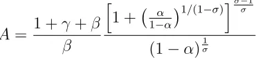
the steady state human capital stock to one, which implies

A= 1 +γ+β

β

h

1 + α

1−_α

1/(1−σ)i

σ−1

σ

(1−α)σ1

Therefore, once we estimate the remainder of the 6 parameters, A is pinned down.10 _{Table 1 recapitulates the definitions of the 6 parameters to be}

estimated.

3.1.1 Data moments

We estimate the parameters using the Simulated Method of Moments as

formalized in Ingram and Lee (1991). Basically we choose moments that

characterize a set of key data features, then search for the parameter values

that minimize the distance between data moments and model moments from 10

It is easy to show that when A is defined like this, human capital stock is convergent.

Based on the estimation results, A is around 11.5 which is not reported in the table of

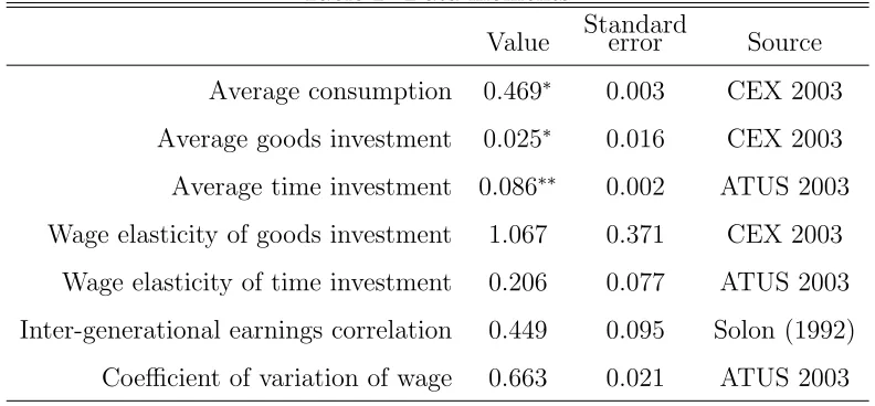
Table 2: Data moments

Value Standarderror Source

Average consumption 0.469∗

0.003 CEX 2003

Average goods investment 0.025∗

0.016 CEX 2003

Average time investment 0.086∗∗

0.002 ATUS 2003

Wage elasticity of goods investment 1.067 0.371 CEX 2003

Wage elasticity of time investment 0.206 0.077 ATUS 2003

Inter-generational earnings correlation 0.449 0.095 Solon (1992)

Coefficient of variation of wage 0.663 0.021 ATUS 2003

* relative to wage/(1-saving rate)

** a fraction of total time available

simulated data. The distance is defined by l2_{-norm, weighted by the inverse}

of the variance of data moments.11

Seven moments are used. Six of them are calculated from the 2003 waves

of the American Time Use Survey and the Consumer Expenditure Survey.

The remaining moment, inter-generational earnings persistence, is taken from

Solon (1992). Table 2presents the data moments and their sources.

The first three moments are the mean levels of consumption, goods

in-vestment and time inin-vestment. These moments pin down the allocation of

parents’ resources. In addition they are informative about the relative

im-11

Ideally we should have used the optimal weighting matrix which is the inverse of the

variance-covariance matrix of the data moments. However the off-diagonal components

are not available from the data, due to the lack of panel data and the fact that moments

portance of time investment in human capital production and the degree of

altruism towards the next generation.

The fourth and fifth moments are wage elasticities of parental investment,

obtained by regressing the logarithm of goods and time investment on the

logarithm of wage rate, instrumented by educational attainment.12

The sixth moment is the inter-generational correlation in earnings.

Ac-cording to Solon (1992), the correlation is around 0.45. This moment is

particularly informative on ρ, the persistence of learning ability over gener-ations.

The last moment is the coefficient of variation in wage rate. This moment

measures the overall wage inequality in the economy. It is very responsive to

the size of random shocks to learning ability. From ATUS 2003, the number

is around 0.66. The literature on economic inequality uses the variance of

logarithm of wage rate as a typical measure of inequality. Since wage rate in

the model is much smaller in scale than in the data, we use the coefficient of

variation so that the model moment is comparable to that in the data.

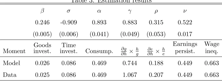
3.1.2 Estimation results

Table 3reports the estimation results. Not surprisingly,σ is negative, which means the elasticity of substitution between goods and time investment is

η = 1 1−_σ =

1

1−₍−_0.909) ≈0.524. The estimate of inter-generational altruism,β,

is 0.246. If we consider one generation to be 20 years, then this is equivalent

12

We use education attainment to instrument wage rate because we want to capture

the human capital element in wage rate. In particular, this filters out shocks to wage rate

Table 3: Estimation results

β σ α γ ρ ν

0.246 -0.909 0.893 0.883 0.315 0.522

(0.005) (0.006) (0.041) (0.049) (0.053) 0.017

Moment invest.Goods invest.Time Consump. _∂h∂g × h_{g ∂h}∂e ×h_e

Earnings persist.

Wage ineq.

Model 0.026 0.086 0.469 0.744 0.188 0.449 0.663

Data 0.025 0.086 0.469 1.067 0.207 0.449 0.663

The table reports estimated parameter values and standard errors.

Mo-ments from simulated data are reported together with those from real

data.

to an annual discount factor of 0.932. Regarding the two parameters for the

unobservable stochastic learning ability process, we find that ρ = 0.315 and

ν = 0.522. Overall our model delivers the data facts very well, except that the wage elasticities of time and goods investment are a little lower in the

model than in the data.

3.2

Inter-generational persistence and wage inequality

Earnings persistence and wage inequality have two sources: exogenous

learn-ing ability and parental investment, which correspond to “nature” and

“nur-ture” effects in the literature respectively. In order to show the roles played

by the latter, we decompose earnings persistence and wage inequality

quan-titatively. First we calculate them in the case in which every individual

makes a steady state level time and goods investment. Next, we keep time

endogenously chosen. Finally, we allow both types of investment to be

en-dogenous. Different results from these cases, reported in Table 4, reveal the

roles played by time and goods investment.

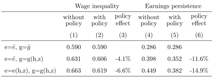
Table 4 shows that parental investment accounts for a relatively small

portion of the wage inequality and earnings persistence. Fixing e and g at the steady state levels, wage inequality is 0.590, while it is 0.663 when bothe

and g are endogenous. Loosely speaking, parental investment, the so-called “nurture effect”, accounts for 11% of overall wage inequality. It accounts for

36.4% of earnings persistence. Within “nurture effect”, both time investment and goods investment are important contributors.13

Table 4: Wage inequality and earnings persistence

Wage inequality Earnings persistence

without

policy policywith

policy

effect withoutpolicy policywith

policy effect

(1) (2) (3) (4) (5) (6)

e=˜e, g=˜g 0.590 0.590 0.286 0.286

e=˜e, g=g(h,z) 0.631 0.606 -4.1% 0.398 0.352 -11.6%

e=e(h,z), g=g(h,z) 0.663 0.619 -6.6% 0.449 0.382 -14.9%

The table reports the decomposition of wage inequality and earnings

per-sistence. The “with policy” case corresponds to an economy where a 5%

income tax is imposed with the revenue invested in public schooling. ˜e

and ˜gare time and goods investment in the steady state.

Columns (2) and (5) of the table report wage inequality and earnings

13

As pointed out by Cunha and Heckman (2007), “nurture effect” and “nature effect”

on inter-generational persistence are nonlinear, and they interact with each other. Our

persistence in the model with public schooling, assuming 5% tax rate. Here

˜

e is still the steady state time investment in the absence of the policy, and ˜

g is defined as public goods investment plus steady state private goods in-vestment. As we allow goods investment to be endogenous and keep time

investment fixed, both inequality and earnings persistence increase, but to

a much less extent compared with the no policy case. Columns (3) and (6)

show the policy effects. Allowing both time and goods investment to be

en-dogenous, the public policy reduces inequality by 6.6% and persistence by 14.9%.

We further decompose the above policy effects by conducting two

ex-periments. Results are reported in Table 5. First, we impose 5% tax, but

assume no public investment in education. This leads to slightly higher

in-equality and persistence, because income tax strengthens the inin-equality in

time investment. In addition, the “tax only” policy leads to slightly lower

time and goods investment. Next, we consider the “public investment only”

policy that keeps public investment from the baseline model unchanged but

assumes away income taxation. The results reveal that much of the policy

effects in the previous discussion are due to public investment, rather than

to income taxation.

3.3

Transition paths

Starting from the original stationary equilibrium, the economy converges to

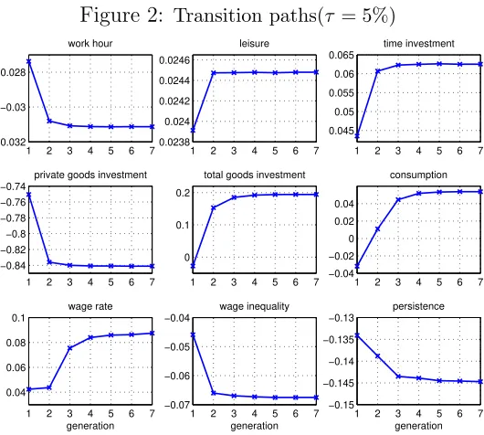
a new equilibrium after the policy is implemented. Given τ = 0.05, we plot the transition paths in Figure 2.

alloca-Figure 2: Transition paths(τ = 5%)

1 2 3 4 5 6 7 −0.032

−0.03 −0.028

work hour

1 2 3 4 5 6 7 0.0238 0.024 0.0242 0.0244 0.0246 leisure

1 2 3 4 5 6 7 0.045 0.05 0.055 0.06 0.065 time investment

1 2 3 4 5 6 7 −0.84 −0.82 −0.8 −0.78 −0.76 −0.74

private goods investment

1 2 3 4 5 6 7 0

0.1 0.2

total goods investment

1 2 3 4 5 6 7 −0.04 −0.02 0 0.02 0.04 consumption

1 2 3 4 5 6 7 0.04 0.06 0.08 0.1 wage rate generation

1 2 3 4 5 6 7 −0.07 −0.06 −0.05 −0.04 wage inequality generation

1 2 3 4 5 6 7 −0.15 −0.145 −0.14 −0.135 −0.13 persistence generation

The figure shows percentage changes due to the implementation of the

public policy. Tax rate is 5%. The top panels plot paths for time

alloca-tion, the middle panels for goods allocation and the lower panels for wage

Table 5: Further decomposition of policy effects Time

investment investmentGoods

Wage rate

Wage inequality

Earnings persistence

(1) (2) (3) (4) (5)

Tax + public inv. 6.1% -84.6% 8.4% -6.6% -14.9%

Tax only -0.8% -4.2% -1.6% 0.4% 0.9%

Public inv. only 6.4% -82.3% 9.1% -6.3% -14.0%

The table reports percentage changes due to different policies. The “Tax

only” case imposes 5% income tax rate, but tax revenue is not invested

in public schooling. The “Public investment only” case keeps public

in-vestment from the baseline model unchanged, but assumes away income

taxation.

tion. The policy shifts parents’ time from work to leisure and human capital

investment. Consistent with the predictions in Proposition I, private goods

investment decreases during the transition, but total goods investment and

wage rate (human capital) increase, which reflects the reinforcing mechanism

among time investment, goods investment and human capital accumulation.

Regarding wage structure, the policy increases average wage rate and

decreases wage inequality and intergenerational persistence. Consumption is

4

Quantitative Results II – the role of time

investment

The reinforcing mechanism illustrated in Figure 1 exists in our model, but

does not exist in the traditional-type model in which parental time investment

is exogenous. Therefore in our model, the policy is much more effective in

promoting human capital accumulation, and in reducing inter-generational

earnings persistence and wage inequality. We quantitatively compare the

policy effects between our model and a version of the traditional model in

which time investment is exogenous.

4.1

The traditional model

We consider a traditional type model that is identical to our baseline model,

except that the human capital production function has the following form

h′ =zA[B + (1−α)(g+P)σ]σ1

Here, we have replaced αeσ _{in our baseline model with a constant B.}

4.2

Comparing policy effects

To compare the policy effects, for each model, we compute the stationary

equilibria in two regimes: with and without public policy, then compute the

percentage changes of variables due to public policy. Differences in results

between the two models reflect the roles played by time investment. Columns

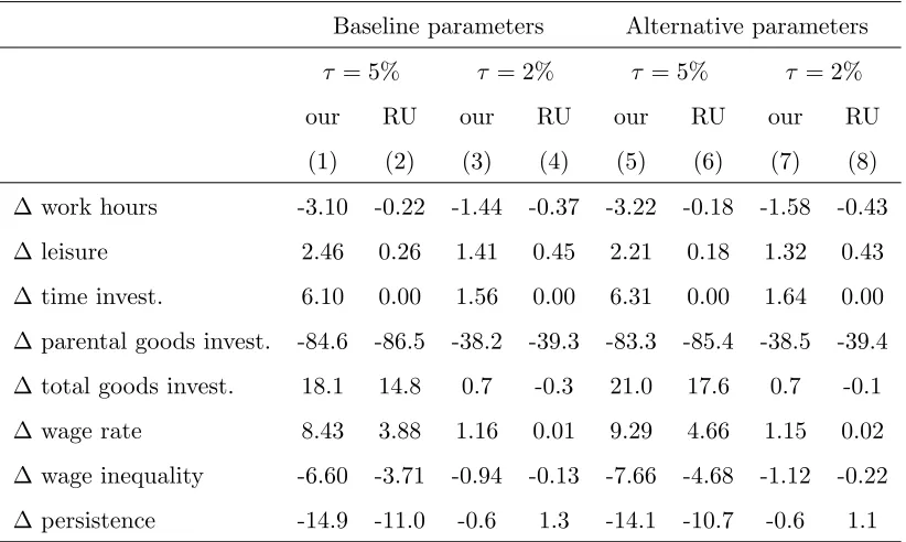
Table 6: Effects of public policy (percentage change)

Baseline parameters Alternative parameters

τ = 5% τ = 2% τ = 5% τ = 2%

our RU our RU our RU our RU

(1) (2) (3) (4) (5) (6) (7) (8)

∆ work hours -3.10 -0.22 -1.44 -0.37 -3.22 -0.18 -1.58 -0.43

∆ leisure 2.46 0.26 1.41 0.45 2.21 0.18 1.32 0.43

∆ time invest. 6.10 0.00 1.56 0.00 6.31 0.00 1.64 0.00

∆ parental goods invest. -84.6 -86.5 -38.2 -39.3 -83.3 -85.4 -38.5 -39.4

∆ total goods invest. 18.1 14.8 0.7 -0.3 21.0 17.6 0.7 -0.1

∆ wage rate 8.43 3.88 1.16 0.01 9.29 4.66 1.15 0.02

∆ wage inequality -6.60 -3.71 -0.94 -0.13 -7.66 -4.68 -1.12 -0.22

∆ persistence -14.9 -11.0 -0.6 1.3 -14.1 -10.7 -0.6 1.1

The table reports policy effects in our model as opposed to the traditional

model (RU) in which parental time investment is exogenous. Columns

(1)-(4) show the comparison based on baseline parameter values (Table3).

Columns (5)-(8) are based on parameter values that minimize the distance

Both models predict a decrease in work hours, which is due to the reduced

after-tax wage rate, but the decrease is more significant in our model where

individuals have the option to make more time investment. Both models

predict increased leisure, and the increase is again much more significant in

our model. Similar changes of time use patterns are found under different

tax rates.

Private goods investment demonstrates huge drops in both models. The

drop is larger in the traditional model. This is because the marginal return

on goods investment is relatively lower due to the inability of individuals

to increase time investment. Total goods investment is increased less in the

traditional model. The policy increases average consumption in both regimes,

but to a greater extent in our model.

Regarding wage structure, the public policy is significantly more effective

in increasing wage rate, and in reducing wage inequality and earnings

persis-tence in our model. With τ = 5%, average wage rate is increased by 8.43%, as opposed to 3.88% in the traditional model. Wage inequality and earnings persistence are decreased by 6.6% and 14.9% respectively in our model, but only 3.7% and 11.0% in the traditional model.

Columns (5)-(8) report the results from an alternative set of parameters

given in Table 7. These are the parameters that minimize the distance

be-tween data moments and moments from the traditional model. Clearly, we

Table 7: Calibration based on the traditional model

β α σ γ ρ ν

0.230 0.854 -0.697 0.883 0.315 0.522

The table reports parameter values that minimize the

distance between data moments and simulated moments

from the traditional model.

5

Further Discussions

5.1

Higher efficiency of time investment by more

edu-cated parents

Ramey and Ramey (2010) point out that more educated parents should be

more efficient in time investment, hence wage/education gradient of parental

time should be positive. We extend our baseline model to admit this

poten-tially important channel.14

5.1.1 Human capital production function and optimal time

in-vestment

Let the human capital production function be

h′_i =ziAα(hδ_iei)σ + (1−α)g_iσ

1

σ ₍₁₄₎

The termhδ

i in equation (14) allows for the channel in Ramey and Ramey

(2010). Since goods investment is absent in their framework, our human

14

We are grateful to a referee for suggestions that led to the development of this

capital production function is essentially the same as in Ramey and Ramey

(2010) if α=1.

When δ = 0, we are back in the baseline model. With non-zero δ, it is straightforward to show the following.

∂gt ∂ht =

1−_σδ

1−_σ

₁−_α

α

_σ−1₁

h

(1−δ)σ σ−1

t + 1

1+γ β + 1

1−_α

α

_σ1

−1 _h (1−δ)σ

σ−1

t + 1

2 (15)

∂et ∂ht =

−(1₁−−δ_σ)σ

1−_α

α

_σ1

−1 _h 1−δσ

σ−1

t

1+γ β + 1

1−_α

α

_σ−1₁

h

(1−δ)σ σ−1

t + 1

2 (16)

Given these equations, there exist two cases in which wage/education

gradients of goods and time investment are positive.

Case (i), δ < 1 and σ < 0. In this case, for parents with more human capital, the efficiency of time investment does not outweigh their advantage

on the labor market. Complementarity between two types of investment is

still needed for the wage/education gradients to be positive.

Case (ii), δ > 1 and σ > 0. In this case, parents with higher human capital are much more efficient in time investment. ∂et

∂ht will be positive if

time and goods investment are substitutes. In addition, from equation (15),

ifδ is large enough, goods investment will decrease with human capital. This is because for parents with more human capital, the advantage in parenting

outweighs the advantage on the labor market, and they substitute goods

investment for time investment.

Since more educated women are more likely to be in the labor force, it is

labor market time more than that of time spent in parenting. Therefore we

focus our discussion on case (i). When the same public policy is introduced

into our model, we find that all the results in proposition I and II hold. The

exception is that the sufficient condition for positive wage gradient of time

investment becomes σ <−₍₁₊β(1_γ−₎₍₁δσ−)_δ).

15

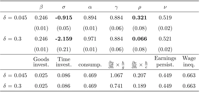
5.1.2 Re-estimation of the model

To conduct a quantitative study based on the extended model, we re-estimate

the model with δ as an additional parameter. The estimation yields δ = 0.045. However, the standard errors ofσ,ρ and δ are large. The model fails to precisely identify time-goods substitutability (σ), persistence in learning ability (ρ) and higher productivity of more able parents (δ), because the product of δ and σ enters the exponential term in the production of human capital.16_{. We proceed by fixingδ at different values and estimating the rest} of the parameters. Generally we find the distance between model and data

moments increases slightly with δ, supporting a low δ.17 _{Table 8 reports} the results with δ fixed at 0.045 and 0.3. When δ is higher, the estimated persistence in learning ability ρ is much lower. Substitutability between

15

Proof of the proposition withδin human capital production function is available upon

request.

16

We thank Dean Corbae for pointing this out.

17

The existing literature provides some indirect evidence in support of a positiveδ. For

example, more educated parents are less likely to use non-parental child care (Leibowitz

(1974a)). Subsidized non-parental care tends to have positive impact on outcomes for

disadvantaged children whose parents on average have lower income and education

attain-ment, but negative impact for children from more educated families. See Blau and Currie

goods and time is also lower, which enables the model to match the positive

wage gradient of goods investment in the data.

Table 8: Estimation results with fixed δ

β σ α γ ρ ν

δ = 0.045 0.246 -0.915 _{0.894 0.884} 0.321 _0.519

(0.01) (0.05) (0.01) (0.06) (0.08) (0.02)

δ = 0.3 0.246 -2.159 _{0.971 0.884} 0.066 _0.521

(0.01) (0.21) (0.01) (0.06) (0.08) (0.02)

Goods

invest. invest.Time consump. ∂g_∂h×h_{g ∂h}∂e ×h_e

Earnings persist.

Wage ineq.

δ = 0.045 0.025 0.086 0.469 1.067 0.207 0.449 0.663

δ = 0.3 0.025 0.086 0.469 0.741 0.189 0.449 0.663

The table reports estimation results for the extended model for two cases,

δ= 0.045 and δ= 0.3. Implied model moments are also reported.

5.1.3 Policy effects in the extended model

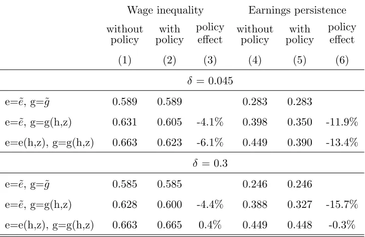
Table9reports the policy effects given different values ofδ. A higherδmeans more of the inter-generational effect is driven by time investment. Compared

with the baseline case, the public policy induces even more parental

invest-ment, hence is less effective in reducing the inter-generational effect. The

table also shows that if time investment is fixed (e=˜e), then policy effects increase with δ.

Table 9: Wage Inequality and earnings persistence from different δ

Wage inequality Earnings persistence

without

policy policywith

policy

effect withoutpolicy policywith

policy effect

(1) (2) (3) (4) (5) (6)

δ = 0.045

e=˜e, g=˜g 0.589 0.589 0.283 0.283

e=˜e, g=g(h,z) 0.631 0.605 -4.1% 0.398 0.350 -11.9%

e=e(h,z), g=g(h,z) 0.663 0.623 -6.1% 0.449 0.390 -13.4%

δ = 0.3

e=˜e, g=˜g 0.585 0.585 0.246 0.246

e=˜e, g=g(h,z) 0.628 0.600 -4.4% 0.388 0.327 -15.7%

e=e(h,z), g=g(h,z) 0.663 0.665 0.4% 0.449 0.448 -0.3%

The table reports the decomposition of persistence and inequality for two

cases, δ = 0.045 andδ = 0.3. Overall policy effects are weaker when δ is

Figure 3: Comparing transition paths from differentδ

1 2 3 4 5 6 7 −0.04 −0.035 −0.03 −0.025 −0.02 work hour δ=0 δ=0.2

1 2 3 4 5 6 7 0.0238 0.024 0.0242 0.0244 0.0246 leisure

1 2 3 4 5 6 7 0.04 0.06 0.08 0.1 0.12 time investment

1 2 3 4 5 6 7 −0.9

−0.85 −0.8 −0.75 −0.7

private goods investment

1 2 3 4 5 6 7 −0.1

0 0.1 0.2 0.3

total goods investment

1 2 3 4 5 6 7 −0.05 0 0.05 0.1 0.15 consumption

1 2 3 4 5 6 7 0 0.05 0.1 0.15 0.2 wage rate generation

1 2 3 4 5 6 7 −0.08 −0.06 −0.04 −0.02 0 wage inequality generation

1 2 3 4 5 6 7 −0.1

−0.05 0

persistence

generation

The figure shows percentage changes due to the implementation of the

public policy, given different value of δ. Tax rate is 5%.

persistence. However, the policy is more efficient in promoting human capital

accumulation, because the reinforcing mechanism illustrated in Figure 1 is

even stronger with a positive δ.

5.2

The substitutability between goods and time

in-vestment

The substitutability between time and goods investment plays a key role in

this paper. In reality, some activities, such as baby sitting, appear to be more

easily substituted by purchased child care. Others, such as breastfeeding, are

the overall substitutability for which there exists little direct evidence. The

observed positive wage/education gradient of parental time can serve as an

indirect evidence. In this subsection we provide a summary of relevant studies

in the literature.18

The literature of home production typically finds a large elasticity of

substitution between goods input and home production time. However, the

production of children’s human capital should be different from usual home

production because time with children has totally different patterns from

other home production time. Due to the lack of direct evidence, some

theo-retical papers assume unit elasticity so that time and goods are combined in

Cobb-Douglas form (Trostel (1993)).

A number of empirical observations imply that parental child care can

be substituted to some extent. Leibowitz (1974a) shows that child care time

is reduced when non-parental child care is present, and such an effect is

most significant among less educated mothers. Government programs that

provide universal day care typically induce more maternal participation in

the labor market, and crowd out some child care time from mothers (Baker

et al. (2008), Havnes and Mogstad (2009) and Gupta and Simonsen (2010)).

On the other hand, there exist a number of empirical observations that

are consistent with a low substitutability.

First, maternal labor market participation only leads to a small-sized

reduction in mother’s child care time, and leads to increased child care time

of fathers (See Leibowitz (1974a), Bianchi (2000), Sandberg and Hofferth

18

We are grateful to a referee for suggestions which led to the development of this

(2001) and references therein). After entering the labor market, mothers tend

to cut back leisure and home production time unrelated to child care, but try

to preserve their time with children. This phenomenon is more pronounced

among more educated women. Using Dutch data, Annemarie Nelen and

Fouarge (2011) even find that maternal working hours are positively related

with planned activities with children, such as going together to a museum or

library.

Second, recent studies revealed the negative impact of maternal labor

market participation on child outcome. Although earlier studies on this

is-sue had reached different conclusions, more recent ones generally document

negative effects. Ruhm (2004) shows that maternal employment has a

nega-tive impact on a child’s verbal ability, and reading and mathematics

achieve-ment.19 _{Bernal and Keane (2011) further document a significantly negative}

and sizeable effect of the increased single mother employment caused by the

1996 Welfare Reform Law along with earlier state policy changes adopted

under federal waivers.

Third, the literature on the correlation between child outcomes and

pro-vision of universal child care programs by governments generally favors a low

substitutability. Baker et al. (2008) use data from Quebec and find that

chil-dren are worse off by a wide range of measures which are likely to be caused

by less and lower quality maternal care. Based on Danish data, Gupta and

Simonsen (2010) show that, compared to parental care, low-quality

non-19

Ruhm (2004) reviewed the existing literature and found that his conclusion is

consis-tent with the most recent analysis , and suggests that the inconsistency with earlier ones

parental care (obtained from so-called family day care) significantly worsens

child outcomes20_{. Havnes and Mogstad (2009) show that the subsidized child}

care program crowds out informal care arrangements from friends, relatives

and unlicensed care givers, leaving parental care virtually unchanged.

Fourth, there exists strong evidence that children with lower birth

or-der (those who are born earlier) have better outcomes. These children on

average receive much more parental time investment than their younger

sib-lings (Price (2008)). On the other hand, they are likely to receive less goods

investment, because parent’s income on average increases with age. The

sig-nificantly better outcomes of children with lower birth order are consistent

with our low substitutability assumption.

From the above discussion, it is not unreasonable to assume that the

sub-stitutability between time and goods is low on average, even though some

parenting activities are clearly more substitutable. Leibowitz (2003) provides

a discussion about why the substitutability appears to be low. First, it is

difficult to monitor the quality of purchased child care. A hired nanny or

babysitter may not spend her time investing in the child’s human capital,

but enjoying her own time at the expense of the child. Secondly, the

psy-chological and sociological literature emphasizes that parent-child bonding

affects child’s development, which is further supported by neurobiologists

(See the references in Leibowitz (2003). Also see Belsky (1988).) Thus, even

for activities such as baby sitting, it is not completely safe to say they can

20

Gupta and Simonsen (2010) also show that enrollment in high-quality preschool does

not lead to significantly different child outcomes, but longer hours in non-parental care

be substituted by purchased care.

5.3

Parental time and public spending on education –

cross country comparison

In Proposition I, we make two predictions regarding parental time and public

spending on education. We roughly check these predictions with cross

coun-try data.21 _{We use the parental time reported in Guryan et al. (2008) and}

public spending on education reported by the World Bank. Figure 4 plots

child care time by working women against public spending on education per

capita. Consistent with proposition I, child care time increases with

pub-lic investment. This relationship also holds for working men. On the other

hand, we find a very weak correlation between education gradient of

parent-ing time by workparent-ing mothers and public spendparent-ing – correlation coefficient

is 0.18 with standard error equals 0.31. In summary we find strong support

for the positive correlation between parental time and public investment, but

little support for the wage gradient of parental time to decreasing with public

investment.

5.4

Other forms of parental altruism

For transparency and tractability, this paper assumes a simple form of parental

altruism – parents care only about the wage rate of their children. In this

21

We are grateful to a referee for suggestions which led to the development of this

Figure 4: Public investment and child care time

0 50 100 150 200 250

4 5 6 7 8 9 10

public spending on education per capita

child care hours −− level

Austria Canada

Chile Estonia

France Germany Italy

Netherlands

Norway

South Africa

UK

US

The figure shows the correlation between public spending on education

subsection we discuss other forms of altruism.22

5.4.1 Financial transfer

We extend our model to admit financial transfer from parents to children.

Let bi be the transfer from the ith parents who maximize max

ci,ni,ei,gi,bi

lnci+γlnni+βlnh′_i+φlnbi

subject to

ci+gi+bi = (1−ei−ni)wi

(17)

Letg∗

and e∗

be the optimal goods and time investment in the baseline

model given {hi, zi}, the optimal goods and time allocation in this extended model is

g = 1 +γ+β 1 +γ+β+φg

∗

and

e= 1 +γ+β 1 +γ+β+φe

∗

Therefore compared with the baseline model, optimal time and goods

investment are reduced by a fixed proportion. As a result, the analytical

properties regarding time allocation and policy effects derived in the

previ-ous sections still hold. Since parents allocate relatively less time and goods

to human capital production compared with the baseline case, the extended

model must attribute a larger part of observed intergenerational persistence

22

We are grateful to a referee for suggestions which led to the development of this

to the “nature effect”, i.e., the persistence in learning ability. Hence

quanti-tatively public policy would be less effective.

5.4.2 Infinite horizon

Another form of parental altruism is to assume that parents care about the

value of their children, which include children’s own utility and the value of

grandchildren. The problem essentially becomes an infinite horizon one with

the following objective function for parents.

max

c,n,e,gE

∞ X

t=1

βtu(ct, nt)

where u(ct, nt) = lnct+γlnnt is the utility of the tth generation, and E is the expectation operator, taken with respect to the learning ability of future

generations.

In this setup, the time-goods investment ratio is the same as in the

base-line model which is e g =

1−_α

α

_σ1

−1 _hσ−11. However, income tax would reduce goods investment to a greater extent23_{. This is because forward-looking}

par-ents care about the future generations’ consumption and leisure which are

directly affected by tax. To see this point, we derive the first order conditions

with respect to time and goods investment given income tax rate τ.

(1−τ)wt

∂u(ct, nt) ∂ct =

∂ht+1

∂et

(1−τ)(1−nt+1−et+1)

∂u(ct+1, nt+1)

∂ct+1

∂u(ct, nt)

∂ct

= ∂ht+1

∂gt

(1−τ)(1−nt+1−et+1)

∂u(ct+1, nt+1)

∂ct+1

It is easy to show that the first order conditions are exactly the same as

those in the baseline model, except for the extra term in brackets which is

23

the marginal value of human capital. In the baseline model, the marginal

value is 1, because parents care about children’s human capital itself. Here,

the marginal value is measured by marginal utility, and lowered by tax rate

τ. Therefore, compared with the baseline case, parental goods investment is reduced to a greater extent. However, the public investment still stimulates

parental time investment due to time-goods complementarity.

6

Conclusion

This paper is motivated by the data observation that parents with higher

wage or education attainment spend more time teaching and taking care of

their children. We show this is consistent with a model of inter-generational

transmission of human capital. A key feature of the model is the low

sub-stitutability between goods and parental time investment in the production

of children’s human capital. We also show that the positive wage/education

gradient of parental investment is reduced by the policy that taxes income

to finance public schooling.

We use the parameterized model to quantitatively study the impact of the

public policy on resource allocation and wage structure. We first show that

parental investment contributes to wage inequality and earnings persistence,

but the contribution is decreased by the policy. Then we derive the

transi-tion paths of the economy from the old equilibrium without public policy to

the new one. The policy leads to increased wage rate, but decreased wage

inequality and earnings persistence. Consumption is decreased initially, but

The public policy triggers a reinforcing mechanism among time

invest-ment, public investment and human capital accumulation. This reinforcing

mechanism does not exist in the traditional model where time investment

is exogenous. Therefore the policy is more effective in our model relative

to a traditional one. This point is made clear as we quantitatively

com-pare the results between our model and a version of the traditional model.

Given the strong evidence that parents use time investment as a means of

inter-generational human capital transmission, we recommend our model as

a framework to analyze relevant public policies.

As an extension to our model we allow parents with more human capital to

be more efficient in time investment. Compared with the baseline case,

pub-lic popub-licy becomes less effective in reducing inequality and intergenerational

persistence, but more effective in promoting human capital accumulation.

We also discuss briefly the implications of alternative forms of parental

altruism. It is worthwhile to study some other extensions. For example,

the model can be enriched by embedding a life-cycle model in the OLG

framework, which facilitates the study of rich dynamics among consumption,

saving and human capital production. This would also allow us to examine

how credit constraints impede human capital formation, and how the

prob-lem can be relieved by public policy. We leave detailed discussion of these

7

Appendix

7.1

Data Appendix

In this paper we estimate the model parameters by matching seven key

mo-ments in the model to their data counterparts. Except for the moment of

inter-generational correlation in earnings which is taken from Solon (1992),

all the moments are obtained from the 2003 waves of the American Time Use

Survey and the Consumer Expenditure Survey.

The American Time Use Survey is conducted by the U.S. Bureau of

La-bor Statistics (BLS) and the data are available from the BLS website. Using

the time use taxonomy introduced in Aguiar and Hurst (2007), we consider

three categories of parental time with children: basic child care, teaching,

and playing. Teaching children includes activities such as reading to/with

children, talking/listening to children, and helping children with their

home-work. Clearly these should be regarded as time investment. Much of the

time categorized as basic child care and playing with children is beneficial

or auxiliary to the development of human capital. For example, “basic child

care” includes activities such as picking up children from school, attending

children’s events; “playing with children” includes playing sports with

chil-dren, doing arts and crafts with chilchil-dren, etc. Therefore we take the sum

of the three categories as the proxy for parental time investment. We proxy

leisure with the time spent on activities related to the following: lawn, garden

and houseplants, animals and pets, socializing and relaxing, sports, exercise

and recreation, telephone calls, household and personal mail, travel related

is precisely “leisure measure two” in Aguiar and Hurst (2007).

Consumer Expenditure Survey data are publicly available from the NBER

collection. Educational expenditure has three categories in the data. The

first one is tuition for college (higher education). The second one is the

tuition for Nursery, Elementary, and Secondary Education. This category

includes tuition for elementary and high school, payment for private school

bus, and other expenses for day care centers and nursery schools. The third

category, other educational service, includes tuition for other schools, rental

of books and equipment and other school-related expenses, and contributions

to educational organizations. We take the sum of the three as the proxy

for goods investment in children’s human capital. The survey provides no

information on whether these expenditures are for children or not, therefore

we delete the observations of families whose head of household is younger

than 25 or not married or have no children. Consumption is measured by

the sum of expenditures on nondurable non-educational goods and services.

We need to calculate educational expenditure normalized by wage rate.

We also need to regress educational expenditure on wage rate to compute the

response of goods investment with respect to parents’ wage rate. Since the

data set provides only family level expenditures, the corresponding wage rate

should also be at the family level. We take wage rate to be the sum of both

spouses’ wage divided by the sum of work hours. i.e.,w= whusband+wwif e

hourshusband+hourswif e.

Note that for both spouses, CEX provides information about annual wage,

weeks worked in the year and hours worked in each week.

In both ATUS and CEX, we delete observations that have one of the