A model of descending auction with
hidden starting price and endogenous
price decrease
Di Gaetano, Luigi
Department of Economics and Quantitative Methods, University of
Catania
1 October 2011
Online at
https://mpra.ub.uni-muenchen.de/39266/
endogenous price decrease
Luigi Di Gaetano
June 6, 2012
Abstract This paper studies a format of descending price auction with hidden price, which is revealed to any participant who pays a participation fee. Each time the price is observed by a participant, it decreases by a fixed amount. Price does not decrease, instead, exogenously. Once a player observes the price, she can buy the auctioned object at the current price. This format has been run on the Internet and is known as ‘price reveal auction’ or ‘scratch auction’.
In the following pages, we will define a model for this format, and derive the Perfect Bayesian Equilibrium for the game. Results are various. Entry in the game is endogenous, players use a threshold strategy to decide whether or not participate the auction. Players find optimal to undercut rivals, because of price endogeneity. Moreover, beliefs about the current unknown price are updated taking into account the time as a signal of the price. If the game continues, players infer that the price is too high and update their beliefs accordingly.
Keywords Price reveal auction·Endogenous price·Descending auction
JEL Classification D44·C72·D82
Department of Economics and Business University of Catania
Corso Italia 55 95129 Catania Italy
1 Introduction
Auctions have always been employed as a method for selling objects since the earliest moment of the human history. During the last years, they were used to sell an increasing number of objects, and different new types of auctions have been modelled to be adapted to various situations.
Several are the factors for these changes. In the first place, the greater deal of attention given by the literature – both theoretical and empirical – of the last decades, have contributed to un-derstand mechanisms which regulate bidders’ actions. Therefore, these improvements constituted also the basis to design new auctions, which had the aim of meeting certain requirements. The technological advantages, on the other hand, had the effect of increasing the number of possible participant of auctions – for instance, by widening the geographical catchment area or increasing the number of bidders – and gave the possibility of organising more complex auction mechanisms. Over the past few years, several new formats are spreading over televisions and the Inter-net; they represent new models of trade, and are different from traditional auctions because of differences in their cost structures and in the organisation rules1.
In this paper we analyse a new auction format, which has experienced some popularity over the Internet, called Price reveal auction (or “scratch auction”). This format consists in a descending auction where (1) the price of the object is not publicly observable, (2) participants have to pay a fee in order to privately observe it, and (3) the price decreases whenever a player observes the price.
The paper is organised as follows. In next section we will discuss about the new pay–per–bid auction formats which are being popular on the Internet, and introduce the related literature. Then, we will introduce a theoretical background for the model of price reveal auctions, analyse its theoretical properties, and derive the predicted best strategies and the perfect Bayesian equi-librium. Due to concealment of the price, we will analyse players’ beliefs and the beliefs updating process. Concluding remarks will follow.
2 New formats and related literature
In recent years, new auction formats have been designed and used online to sell objects. For their characteristics, they cannot be collocated in the standard literature about auction (such as Klemperer 1999; Krishna 2002; Menezes and Monteiro 2005).
Among these, the most common new formats are Penny auction, Lowest unmatched bid auction and Price reveal auction (also known as scratch auction). There are four main factors which are common among these formats: (1) Players pay a fee to participate the auction or to submit their bids and entry is endogenous; (2) the auctioneer raises his revenues through fees, perhaps, the winning bidder could pay a relatively small price to but the object; (3) although the simplicity of the formats, game theoretical analysis results to be complex and often equilibria are derived using numerical simulations (Houba et al. 2011); (4) finally, they are relatively recent online auction formats, and this is reflected in the related literature.
In lowest unmatched sealed bid auctions, a generic player wins the object if she submits the lowest bid which is also unique (i.e. there does not exist another player who has submitted a bid of the same amount). Players pay a fee to submit their bids, and entry is endogenous.
This format has been analysed by Houba et al. (2011); Östling et al. (2007); Eichberger and Vinogradov (2008); Rapoport et al. (2007). The complexity of the strategic space, however, has
1 See, for example, Gupta and Bapna (2001) for a review of the principal online auction mechanisms and of the
forced authors to analyse the format using some restrictive assumptions. Östling et al. (2007) and Rapoport et al. (2007), for instance, assume submission fees to be zero.
Eichberger and Vinogradov (2008) find that there is not a Nash equilibrium in pure strategies in their model of lowest unique bid auction, and they characterise the equilibrium in mixed strategies. However, they find also that data do not fit the predicted optimal strategy.
Houba et al. (2011) focus, instead, mainly on theoretical issues, such as the endogenous entry of players – which creates uncertainty on the number of participants – and on how players bid in least unmatched bid format. They analyse symmetric equilibrium of the game, by assuming that player can submit only one bid, while in reality multiple bids can be submitted. Results are several, symmetric equilibrium in the auction with more than two players is the maxmin
equilibrium, while with two players the format is strategically equivalent to the Hawk-Dove game.
The format usually known as penny auction has been analysed by Hinnosaar (2010) and Augenblick (2009). In this auction, each bid increases the price of the object, similarly to an English auction. Bids are costly, and a player wins if she submits a bid and no other bids are submitted before a certain amount of time. For its characteristics, it is similar to a war of attrition game (Hinnosaar 2010). In this format, however, players pay a fee only to submit a bid, so they can choose to remain inactive for a certain period of time.
Both Hinnosaar (2010) and Augenblick (2009) derive the equilibrium of the game and compare results with empirical observations. Hinnosaar (2010) finds that“in the increasing price auctions, the upper bound of possible prices isp= [v−c]−1 +N and it is reached with positive probability. This is a very high price where even the winner gets strictly negative payoff”. Augenblick (2009) analyses the equilibrium hazard rates of penny auction and the mixed–strategy equilibrium. He, then, compares his results with empirical data, finding that auctioneer’s revenues are usually higher than the objects’ market value and that the starting hazard rate is similar to predictions, but it decreases in time. Moreover, He shows that data fits his prediction of sunk cost fallacy, since players submit several bids. Players’ learning process determines the exit from the game, although it happens after huge losses.
The last format is price reveal auction, alternatively known as scratch auction. This format is a descending price auction, where the price is hidden for bidders – who have to pay a fee in order to observe the price and buy the object – and the price decrease mechanism is endogenous. Because it is a descending price auction, it is apparently similar to a Dutch auction. However, in this format, the price is hidden and decreases not because of the time, but because of players’ actions (endogenous price decrease mechanism). The two principal websites which offer this format are Bidster.com and Dealwonders.com.
To better understand how this auction mechanism works, we can quote the description of the auction rules of one of the websites which organises this auction format. Bidster.com organises “scratch auction” since the 29th December 2009 (Gallice 2010), the auction is defined as follow:
“On Bidster’s Scratch Auctions the current price is hidden from the participants until the participant scratches the auction. Then the participant will see the current price. Every time someone scratches the auction the price is lowered. So the more people that scratch the auction the faster the price will drop. [. . . ]
Auction example (Scratch auction): The market price of the product is £ 100. Starting price for the auction is £ 95 (the start price is hidden for the participants). Every scratch lowers the price £ 2.5.
current price £ 85.00. She thinks it’s a good price and chooses to purchase the product. Then the auction ends and Maria is the winner.”2.
To the best of our knowledge, we are aware of only one contribution to the literature with regard to this format (Gallice 2010). Gallice (2010) develops a model where the price is hidden in each period. The starting price is set equal to the retail price of the object, and he assumes that players’ valuation are distributed between zero and the retail price. Players could observe the price or not. After observing it, they decide to buy the object or not. To observe the price they should pay a feec. Every time someone observes the price, it is decreased by a value smaller thanc. The price, in Gallice (2010), decreases only for this reason.
Gallice (2010) derives a very clear prediction for the (unique) perfect Bayesian equilibrium. According to his model, every player decides not to observe the price and the auctioneer’s revenues are zero. Since the starting price is known and equal to the maximum valuation and due to the presence of the costc, it is not optimal for the player with valuation equal to the retail price to observe the price. Consequently, the price does not decrease, and players with lower valuations do not find optimal to participate the auction as well.
The result is that no one observes the price. However, these results – as the same author observes – are not consistent with empirical data.
As we will sin next sections, due to the hidden price and the bidding fee, the entry of players is endogenous. Moreover, since the price decreases because of the action of players, the price decrease mechanism is also endogenous.
The problem of endogenous entry of players in standard auction setting was studied by Levin and Smith (1994), McAfee and McMillan (1987), Menezes and Monteiro (2000) and Chakraborty and Kosmopoulou (2001). In particular, Menezes and Monteiro (2000) study the case in which players known only their valuation and the potential number of participants. They introduce a threshold strategy according to which only bidders who have a valuation above a certain cut-off value submit a bid. They, consequently, derive the optimal bidding functions for first price and second price sealed bid auctions.
3 A model of price reveal auctions
In this section we develop a model for price reveal auctions. The basic mechanism of this auction format is the following. Players do not know neither the starting price of the object auctioned, nor the current price at each time. Moreover, they do not know the number of players who have observed the price previously. A generic player has to pay a fee to observe the price, then he has to decide to buy the object or not. Price decreases whenever a player observes it.
3.1 The model
The model of price reveal auction consists in a sale of a unique and indivisible object.
There areI ={1,· · ·, n} risk neutral bidders. Each player has ani.i.d.private valuationvi, distributed according to a generic cumulative distribution function (cdf)F(·) – and probability density function (pdf)f(·) – over the support [0,v¯]. The distribution is non decreasing, continuous and differentiable.
At timet= 0, nature selects players’ valuations. The game starts att= 1 and it stops at T
or if a player buys the object.
The price is hidden at each timet. Moreover, the initial pricep0is randomly chosen by nature.
We assume that the auctioneer is always willing to trade.
The starting price is defined asp0=α, where αis a random variable. It is distributed over
the interval [α, α] according to acdf G(·) (and apdf g(·)). The distribution ofαand its support, are known by all players. The starting price could be above the highest valuation ¯v,i.e.it could be the case thatα >¯v.
The price of the object decreases, by a positive quantity δ, if only if a player observes it. Consequently, in each t, the price is pt =p0−δηt, where ηt ∈ N is the number of times the price has been observed up to timet. We need to remark that, as in the actual auction format, the price decreases when a player observes it and, therefore, a generic playeriobserves the price already lowered.
Players do not known the price before observing it. Furthermore, they do not know how many players have observed the price before (i.e.ηtis unknown).
At each time t≥1 – in the same fashion of Gallice (2010) – a generic playeri has a set of strategies Ai,t ={nobs; (obs, b); (obs, nb)}, (∀i ∈ I). Players can decide to observe the price or not, after having observed it, they choose to buy the object or not. If a player observes the price and does not buy the object, she will exit the game. To observe the price, bidders pay a feec >0 (c > δ) to the auctioneer.
The payoff of a generic player with valuationvi is:
πi =
vi−pt−cif playeri observes and buys the object (at timet) −c if playeri observes the price and does not buy the object
0 otherwise
(3.1)
This setup shares several characteristics with that of Gallice (2010). There are, however, some different assumptions.
The starting price is a random variable and is hidden to buyers, while in Gallice (2010), the initial price was known and set equal to the retail price.
The concealment of the starting price reflects the real auction format3. The starting price,
moreover, is random and could be greater than ¯v.
A central assumption is that each player can observe the price, and buy the object, only once. This is indeed a strong assumption, which does not reflect the actual format. However, it is necessary to derive the Perfect Bayesian Equilibrium in the game. We will comment this assumption later, and explain why it is a central assumption and how it can affect theoretical findings.
3.2 Optimal strategy and second stage decision
Randomness and concealment of the starting price in our auction format, together with the fact that players are allowed to refuse to buy the object, are critical points of the analysis of the optimal strategies.
Gallice (2010) introduces a threshold strategy based on the fact that refusing to buy the object – after the observation of the price – is not optimal in his model. According to his considerations, the strategy (obs, nb) is dominated and never chosen. Thus, he argues that the equivalence between first price auction and Dutch auction could be used as platform for building players’ beliefs and strategies.
In our case, since the starting price could be above bidders’ values, we cannot exclude the strategy (obs, nb). However, we can separate players’ strategies in two stages: in the first one,
they choose whether observing the price or not, in the second – conditional on observing the price – they decide to buy or not the object.
The second stage decision trivially depends on the known price. Since players can enter the auction (observe the price) only once, they will decide to buy the object if the actual price is below their valuations.
Proposition 1 Conditional on observing the price, player i will buy the object if the price is below her valuation, i.e. ifvi≥pt
Proof Conditional on observing the price, playerihas already sustained the entry feec, thus it is a sunk cost. If she buys the object, she receives a payoffvi−pt.
Since each player can observe the price (and buy the object) only once, the payoff associated tonbis zero. Therefore, the strategy (obs, b) dominates (obs, nb) ifvi−pt≥0. Playeriwill buy the object ifvi≥pt.
3.3 First stage decision
The standard Dutch auction format, in the simplest setting with private valuations, is strategi-cally equivalent to a first–price sealed bid format. A generic player is willing to stop the auction whenever the price is equal to (or smaller than) her optimal bid in the equivalent first price auction; because a generic player maximises her expected payoff, given that no one has stopped the game before.
In our model, differently from the standard Dutch auction format, players can observe the price and refuse to buy the object. Therefore, the game can continue also if someone has already observed the price. This is a central consideration, which should be taken into account when deriving the optimal strategy.
Proposition 2 Suppose that each player j 6= i follows a strictly decreasing and continuous strategy t(vj), which maps every valuation with a period t in which is optimal to observe the
price. Suppose also that playeridecides to follow a strategy t(x), for an arbitrary valuex. Then, if a playerk (k6=i) observes the price beforei and the game continues, we have that the price (already decreased) is greater thanvk> x.
Proof Player k will not buy the object if the price, which she observes, is greater than her valuation (second stage decision). Moreover, if a playerkobserves the price beforei, it must be the case thatvk> x4. Consequently, we have that the price is higher than vk andx.
If someone has observed the price and refused to buy the object, player i infers that the price is greater than her private value. Proposition 2 has two main consequences on players’ strategies. On the one hand, beliefs about the current price must be updated taking into account the possibility that people can observe and refuse to buy the object. On the other hand, player
ibases her maximisation problem on the probability that no one has observed the price before, otherwise, she expects her surplus to be negative.
Hence, is not optimal to observe the price if someone has observed the price beforet(x) (for
x=vi).
A generic playeri will maximise the following expected utility:
max{[vi−pt(t(x))]·P r(t(x)≤t(vj),∀j6=i) ; 0} −c (3.2)
4 t(·) is a (strictly) decreasing and continuous function and we have thatt(vk)< t(x) ⇐⇒ v
maxn[vi−pt(t(x))]·F(x)n
−1
; 0o−c (3.3)
The expected utility is derived as follows. Given that all playersj – with j 6= i – follow a strategy t(vj), and player i has a strategy t(x). If no one has observed the price before – with probabilityF(x)n−1
– the expected surplus is positive. On the opposite case, the expected surplus in negative andiprefers not to buy the object (the the payoff is simply zero). Furthermore, the feecmust be taken into account.
Note also that, since the price decrease mechanism is endogenous, the price does not decrease because of the time. And, for this reason, we have thatp′
t= 0
First order condition for the problem is derived by taking the derivative with respect tox, and imposing it equal to zero:
maxn[vi−pt(t(x))]·(n−1)f(x)F(x)n−2−pt′(t(x))F(x) n−1
; 0o= 0 (3.4)
it should be optimal for x=vi:
maxn[vi−pt(t(vi))]·(n−1)f(vi)F(vi)n−2−pt′(t(vi))F(vi) n−1
; 0o= 0 (3.5)
We find the usual condition for a Dutch auction, but we should consider also that p′
t = 0, therefore we have that:
max
[vi−pt(t(vi))]·(n−1)f(vi)F(vi)n−2; 0 = 0 (3.6)
According to the FOC, players are willing to observe the price as long as they expect it to be equal to their valuations. Due to price decrease mechanism, players do not find profitable to wait, because the price is not expected to decrease, and there are only possible losses due to the fact that someone could observe the price and buy the object.
Note that this is a necessary, but not sufficient condition. In Appendix A we derive the same result using different arguments.
In the usual Dutch auction format, there is a trade off between the expected marginal gains of waiting the price to decrease (represented by the lower price in the future) and the marginal expected losses due to the lower probability of winning the auction. In our model marginal gains are zero. Since the price decreases if players observe it, either the price is too high or the object is bought by another player.
In this setting, consequently, players always find optimal to undercut their rivals, as long as the expected price is smaller than – or equal to – their valuations. Moreover, we should also consider the feec.
Remark 1 Given the expected price at timet, the probability of buying the object, which makes a generic player indifferent between the actionsobsandnobs, is:
[vi−pet]P r(pt≤vi)−c= 0 ⇐⇒ P r(pt≤vi) =
c vi−pet
(3.7)
In the left hand side, we have the expected utility of the actionobs, that is the expected payoff times the probability of buying the object5 and the participation feec. While in the right hand
side, zero represents the payoff of the action nobs.
Proposition 3 The optimal (first stage) strategy for a generic playeriis to observe the price if
pe
t≤vi−c and if P r(pt≤vi)≥vi−cpet
Proof Players are willing to undercut their rivals, due to endogenous price decrease mechanism, and observe the price as soon as the expected price is below or equal to their valuations.
Since a feecis paid to observe the price, the strategyobsis not optimal whenpe
t =vi. Player
iwill observe the price ifP r(pt≤vi)≥ vi−cpet, which corresponds to the case where the expected
utility ofobsis greater or equal to that ofnobs, given player’s beliefs.
Moreover, since a probability is always included between 0 and 1, we have also that 0 ≤ c
vi−pet ≤1. Which means thatvi−p
e
t >0 andvi−pet ≥c ⇐⇒ pet ≤vi−c.
3.4 Qualification of Perfect Bayesian equilibrium
Given previous considerations, we can define the PBE of the game.
Proposition 4 A perfect Bayesian equilibrium of the game consists in n sequences of actions
a∗
i,t T
t=1 (for everyi∈I) where a ∗
i,t is playeri’s optimal strategy at timet:
a∗i,t=
(obs, b) if µi,t=P r(pt≤vi)≥vi−cpet andvi−pt≥0
(obs, nb)if µi,t=P r(pt≤vi)≥vi−cpet andvi−pt≤0
(nobs) if µi,t=P r(pt≤vi)<vi−cpet
(3.8)
WhereP r(pt≤vi)represents playeri’s beliefs about the current price andpet is the expected
price at time t.
Proof The PBE of the game derives from first and second stage decisions. The action nobs
dominatesobsifP r(pt≤vi)<vi−cpet, and is dominated otherwise.
Conditional on observing the price, the decision of buying the object depends on vi and pt, as long as the former is greater than (or equal to) the latter, playeriis willing to buy the object,
i.e.(obs, b) strictly (weakly) dominates (obs, nb).
There is not a separating equilibrium of the game. This means that, given expectations about the price, there will be either no one or a bunch of players who are willing to observe the price.
In particular – when the game starts – ifpe
1=E[α]≥¯v, no one will enter the auction (since
the expected price is higher or equal to the highest valuation and players should sustainc). The same happens ifE[α]<v¯andP r(p1≤¯v)<v¯−Ec[α].
Suppose instead that there is a value ˙v such that 0< v <˙ v¯ and P r(p1 ≤ v˙) = v˙−Ec[α]M.
Since ∂P r(p1≤v)
∂v ≥0, and∂
c
v−E[α]M/∂v <0, all players with valuations between ˙v and ¯v will be willing to observe the price.
4 Characterisation of beliefs
There are different considerations to do when analysing players’ beliefs. In periodt= 0, players receive their own signals (their valuations) and have no other information at their disposal.
In periodt= 1 the game starts. Therefore, no one has observed the price before – i.e.η1= 0
– and the expected price att= 1 ispe
1=E[α]6.
Due to the randomness of the initial price they formulate their beliefs – for the first period – as follows:
P r(pt≤vi|t= 1 ) =P r(α≤vi) =G(vi) (4.1)
6 WhereE[α] is the expected value ofαand is equal toE[α] =Rα
Where G(·) is the cdf of α. Each player i holds beliefs, at time t = 1, represented by the probability thatαis belowvi.
Definition 1 A generic player iwith valuationvi holds beliefs at timet= 1 equal to:
µi,1=
G(vi) ifα≤vi≤α
0 otherwise (4.2)
For everyt > 1, and until the game is finished, beliefs are updated using new information. Players consider the information that the game is still continuing as a signal of the current price. The game continues for two reasons. Either no one has observed the price – and the price is not expected to decrease – or some players have observed the price but they refused to buy the object because the price was too high.
This is a central characteristic of the model. Time is a signal about the price. Moreover, it is a bad signal because the greater is the time elapsed the bigger is the expected price.
To define beliefs fort≥2, we must introduce two definitions. First of all, players do not know the number of opponents who have observed the price previously. Players, moreover, infer that only opponents with certain characteristics (i.ewith valuations greater than a certain threshold) have observed the price before.
Definition 2 Define ξt=E(ηt) as the expected number of players who decide to observe the price up to periodt. Note that, since players are rational,ξ1=η1= 0.
There is no publicly observable information about the number of players who have already observed the price. Therefore, a generic player i substitutes the missing information with the expectation defined above.
Remark 2 In each periodt, given beliefs about the price, all players with valuation between ˙vt and ¯v will observe the price, while players with valuation below the former will not. Where ˙vtis defined as follows:
˙
vt:P r(pt≤v˙t) =
c
˙
vt−pet
(4.3)
Beliefs are not decreasing with respect tov, i.e. ∂P r(pt≤v)
∂v ≥0, and
∂ ∂v
c v−pe
t
<0. Therefore, there is a value which satisfies the equality which has the following properties: for values below it, the LHS is smaller than the RHS, and players with those private values are not willing to observe the price. For values above it, all players will be willing to observe the price; since the LHS is greater than the RHS.
The above definitions are needed to define the information updating process of players. If someone is expected to observe the price in the previous period and the game is continuing, players will update their beliefs thinking that the price is higher than a certain valuation. Given the absence of information, they compute the expected maximum valuation, defined as follows.
Definition 3 Define the valuevmaxe|t as the expected maximum valuation conditional onvi≥v˙t. That is the expected value of the highest order statistic, conditional on having values above ˙vt. It is equal to:
ve|t
max=
1 1−F( ˙vt)n−1
Rv¯
˙
vtx·nF(x)
n−1
f(x)dxif ˙vt<v¯
¯
v otherwise
(4.4)
If the game continues and players expect that someone has observed the price in the previous period, they infer that the price is expected to be higher thanvemax|t−1. Then we can define beliefs fort≥2
Definition 4 In a generic periodt≥2 beliefs are:
µi,t =
µi,t−1 ifξt=ξt−1
[G(δξt+vi)−G(δξt−1+v
e|t−1
max )]
1−G δξt−1+v
e|t−1
max
ifξt> ξt−1 and this number is positive
0 otherwise
(4.5)
Whereξtis the expected number of times the price was observed up to timet(withξ1= 0) and vmaxe|t is the expected maximum valuation at timetas defined above.
Proof See Appendix B for derivation.
5 Remarks
In our model of price reveal auction, we found that players are willing to undercut their rivals and observe the price as soon as it is expected to be below or equal tovi−c(and ifP r(pt≤vi)≥
c vi−pet).
This behaviour is a consequence of the endogenous price decrease mechanism. Since players do not expect the price to fall from time to time – because they want to observe the price only if they expect to buy the object – they do not have any incentive in waiting.
In a standard Dutch auction, this incentive is represented by the price decrease, which creates a trade–off between lower probability of winning the auction and bigger (positive) difference between players’ valuation and price. Thus, players can find optimal to observe the price, and buy the object, if the price is greater than the optimal price in Dutch format (and conditions underlined above are met).
Moreover, entry in the game is stimulated by the randomness of the starting price, together with its concealment. Incentives in entering the game, however, decrease with time, because players update their beliefs and expect the price to be higher if someone has not still bought it. The fact that the game is still continuing is a bad signal for players. Because it means that (if initial beliefs are such that someone is expected to observe the price) the price is higher than the valuation of players who observed it.
Although incentives of observing the price may exist in the initial phases of the game, they decrease overtime and disappear after a certain period. This is the effect of the beliefs updating process, which uses time as an information about the concealed price. Similarly to the information
“winning the game” in the winner’s curse in common value auctions, the information“the game continues” is a bad signal for players, because they are informed about the (high) level of the price. Consequently, beliefs are updated accordingly.
In Gallice (2010), in equilibrium, players decide not to observe the price in each period. In our model, however, is theoretically possible to sustain an equilibrium where some players are willing to observe the price at least in the first place. Our result is coherent with the existence of the online auction format, since empirically players do participate the auction.
The auctioneer finds profitable to increase the number of participants (who observe the price), rather than selling the object with the highest possible price. This because revenues are raised through participation fees and the selling price. Moreover, whenever a player observes the price the auctioneer gainsc−δ >0.
Players can observe the price only once. This is a strong assumption, which does not reflect the real format. However, it is necessary to derive the PBE. By removing this assumption, second stage decision (buy or not buy the object) depends on expectation of future prices, which is an endogenous variable (because it depends on players’ optimal strategies); so it is necessary, due to complexity of strategic space, although it affects the power of our model of explaining empirical observations.
6 Numerical examples and empirical observations
In this section we will show a simple example of the game. Suppose that there aren= 4 players, withi.i.d.uniformly valuations distributed over the interval [0,1]. Furthermore, assumeαto be distributed uniformly between [0.1,1.1]. Therefore, its expectation isE[α] = 0.6 andpe
0= 0.6.
To simplify our analysis, assume that players have the following valuations7:v
1= 0.8,v2 =
0.6,v3= 0.5 andv4= 0.1. We will observe three cases.
First case
Suppose that the realization of αis 0.9, so the (concealed) starting price is equal to this value. Assume the value of δ to be 0.05, while the participation fee is equal to c= 0.12. In this case, participation fees are relatively big (about 10% of the upper–bound in the valuations support).
Remark 3 At time 1, all players with valuation over ˙v1= 0.82 will observe the price. Where this
value is derived as follows (using expression 4.3):
˙
vt:P r(0.6−0.05≤v˙t) = v˙t−(00..612−0.05)
˙
vt: 1−0.55 = v˙t0−.120.55
˙
vt= 0.82
(6.1)
No one, therefore, will observe the price. However, beliefs are updated taking into account that the number of observed is not a public observable information. At time 1, no one is expected to observe the price (ξ1≈0)8. So beliefs do not change and no one will observe the price.
High participation fees, and the particular realisation of valuations –i.e.no one has a private value higher than 0.82 – leads to non participation.
Second case
Assume now thatc = 0.01 and δ= 0.005. Now fees represents 1% of the higest valuation. The realisation of αis, again, 0.9.
7 Which is a private information 8 Note thatξ
1is the expectation ofη1and is derived as the expected number of players with valuations between
Remark 4 At time 1, all players with valuation over ˙v1 = 0.625 will observe the price. Where
this value is derived as follows (using expression 4.3):
˙
vt:P r(0.6−0.005≤v˙t) =v˙t−(00.6.01−0.005)
˙
vt: 1−0.595 = v˙t−0.001.595
˙
vt= 0.62
(6.2)
In this case, player one will observe the price, since it has a valuation above 0.62. However, he will not buy the object because his surplus is smaller than zero. This because, the starting price is
p0=α= 0.9, when player 1 observes the price he will see the pricep= 0.9−0.005 = 0.895>0.8.
Moreover, as before, no one is expected to observe the price,i.e.ξ1≈0.
Lower fees stimulate entry. The concealed starting price, however, is too high and no one will buy the object. Players update their beliefs and expect the price not to change significantly, so they do not observe the price.
Third case
Assume c = 0.01, δ = 0.005, and α= 0.7. The value ˙v1 = 0.62 does not change. Player 1 will
observe the price also in this case. Moreover, he will buy the object, since its surplus is positive (p= 0.7−0.005 = 0.695<0.8). The auction will end in first period.
These three examples are useful to explain the characteristics of the model. Randomness of initial price stimulates entry of players, who observe the price also if the unknown realisation is too high. Therefore, the distribution can avoid entry of players regardless to the actual realisation (as, for instance, in the first case if we supposeα= 0.2).
Participation fees have an important role in entry of players. Finally, beliefs are updated, and time is considered a bad signal in our model. Players learn not to observe the price because they expect an high price.
6.1 Empirical observations
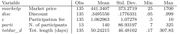
Finally, we must consider empirical results from the online auctions. Table n. 1 shows some summary statistics about all price reveal auctions held in Bidster.com between the 4th January 2010 and the 26th April 2011.
Variable Obs Mean Std. Dev. Min Max
marketp Market price 135 441.3407 373.2719 25 1700
disc Discount 135 .3495556 .1776331 .05 .999
c Participation fee 135 1.062963 1.07278 .5 10
parti N. of participants 13 140 86.93197 7 325
[image:13.595.166.473.542.601.2]totdur_d Tot. length (days) 135 50.24215 46.48102 .17 307.83
Table 1 Descriptive statistics of all paying price reveal auctions ran in Bidster.com and ended between the 4th
January 2010 and the 26th April 2011
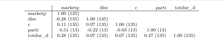
marketp disc c parti totdur_d marketp 1.00 (135)
disc -0.28 (135) 1.00 (135)
c 0.11 (135) 0.07 (135) 1.00 (135)
parti 0.51 (13) -0.22 (13) -0.03 (13) 1.00 (13)
[image:14.595.91.468.92.159.2]totdur_d 0.28 (135) 0.07 (135) 0.07 (135) 0.47 (135) 1.00 (135)
Table 2 Pairwise correlation matrix for all paying price reveal auctions ran in Bidster.com and ended between
the 4th January 2010 and the 26th April 2011 (N. of observations in brackets)
Our prediction is that players can observe the price, but the longer is the time elapsed the lower are players’ incentives of observing the price. Thus our model does not properly explain the average duration of the game.
Furthermore, it is interesting to look at the pairwise correlation matrix (Table n. 2). The market value of objects is positively correlated with the number of participants and, consequently, negatively related with the discount.
Participation fees have a negative correlation with the number of entries in the auction. This is consistent with the threshold rule derived in our model (expression 4.3) and with our numerical examples.
Our theoretical results, however, does not perfectly match with empirical observations. This is principally due to different assumptions of our model. As said in the first pages of this paper, the difference between empirical observations and theoretical predictions is a problem which is present in other studies about all new formats of auctions9.
Moreover, Gallice (2010) has explained differences between predictions and actual data by arguing that the main cause is bounded rationality. Although, it could be reasonable to allow for bounded rationality, these differences are also due to our assumptions. Removing them, however, leads to the absence of an equilibrium.
7 Conclusions
We develop a model of descending auction with hidden price and endogenous price decrease. In this auction format, known as price reveal auction, the price is hidden in each period and decreases if only if players observe the price. Our model is theoretically based on the model of Gallice (2010). He assumes the starting price to be known by all bidders and equal to the market value of the object (which is also equal to the highest value of players’ valuations’ distribution ¯
v).
We introduce, instead, a hidden starting price, to fit better the format which is run on the Internet. We define the starting price as a random variable, which can assume values also above the highest players’ valuation (¯v).
Players’ strategies are divided in two stages: decision of observing the price or not, and – conditional on observing the price – decision to buy or to exit the game. However, we assume that players could not observe the price – and buy the object – more than once.
Our results have some interesting characteristics. First of all, we find that, due to the endoge-nous price decrease mechanism, players do not have any incentive in waiting. They, therefore, are willing to observe the price as long as it is expected to be below their valuations. This result differs with respect to a standard Dutch auction, where players wait until the price reaches the optimal bid of an equivalent first-price sealed bid auction.
9 See Gallice (2010); Houba et al. (2011); Östling et al. (2007); Eichberger and Vinogradov (2008); Rapoport
Moreover, we find that it is possible to have an equilibrium with some players who observe the price, at least in the first period. This result is different from Gallice (2010), who finds that players do not observe the price because of their beliefs. Our findings could explain partially the empirical observations, because entry is theoretically possible.
In our model there is not a separating equilibrium. Given beliefs and players’ characteristics, in each period there will be either no one or a group of players who are willing to observe the price.
Future developments are represented by the possibility of allowing boundedly rational players, and of analysing efficiency properties of the format.
Appendix
A First stage decision
We can derive the same result in expression (3.6) using different arguments. The strategyt(vi) is optimal for playerias long as she finds profitable to observe the price int(vi) instead oft(vi) +dt.
Att(vi), playerihas an expected payoff of max [vi−pt; 0].
Att(vi) +dt, two possible cases should be considered. If no one has observed the price, the price does not change. The probability of this case is 1−(n−1)f(vi)F(vi)n−2 dt
t′(vi)
10. So with this probability the price does
not change.
If another player, instead, observes the price, there are two possibilities. If she buys the item, then playeri
payoff would be zero. If she does not buy the item, for Proposition 2, playeriinfers thatpt(vi)+dtis greater than
her valuation and, consequently,pt(vi)+dt> vi. Therefore the surplus is negative.
So the optimal condition is:
– When the price is greater thanvi, the optimal first order condition is 0 = 0 (always satisfied). – When the price is smaller than (or equal to)vi, betweent(vi) andt(vi) +dt, with probability
1−(n−1)f(vi)F(vi)n−2 dt t′(vi)
no one observes the price and it does not change. With the complementary probability someone (with valuation equal to vi) observes the price and buys the object. And the optimal condition is:
max{vi−pt; 0}= max
n
[vi−pt]
h
1−(n−1)f(vi)F(vi)n−2 dt
t′(vi) i
; 0o (A.1)
which becomes (we can remove the max operator because we supposed thatpt≤vi):
[vi−pt]
h
(n−1)f(vi)F(vi)n−2 dt
t′(vi) i
= 0 (A.2)
The left hand side represents the marginal cost of waiting untilt(vi) +dt, while 0 represents the marginal gain from waiting. It is optimal to stop att(vi) if the marginal cost of waiting (not observing the price) is greater or equal to the marginal gain of not stopping (the LHS is greater or equal to 0).
Players are willing to observe the price as soon aspt≤vi11, because they do not expect the price to decrease exogenously. Note that this is only a necessary condition, which does not take into account the feec.
B Definition of beliefs
When no one is expected to observe the price in previous period,i.e.ξt=ξt−1, price does not change, and beliefs
remain stable overtime.
Ifξt> ξt−1beliefs are updated as follows12:
10 That is the complementary probability of the event in which a player with a valuationv
iobserves the price betweent(vi) andt(vi) +dt.
11 Since the price is hidden, players will use the expected price at timetdenoted aspe t
12 Note that we are applying Bayes rule:P(A|B) = P(A∩B)
P rpt≤vi
t, vi, pt−1≥v
e|t−1
max
=P rα−δξt≤vi
t, α−δξt−1≥v
e|t−1
max
=hG(δξt+vi)−G
δξt−1+vemax|t−1
i
/h1−Gδξt−1+vemax|t−1
i
(B.1)
Bidders use the information “no one has bought the object” as a signal of the possible value of the price. This formula is negative whenδξt+vi< δξt−1+vmaxe|t−1, thenµi,t= 0.
References
N. Augenblick.Consumer and Producer Behavior in the Market for Penny Auctions: A Theoretical and Empirical Analysis. mimeo, Stanford University, 2009.
Bidster.com. Scratch auction: how it works, June 2011. URLhttp://www.bidster.com/page/how-it-works. I. Chakraborty and G. Kosmopoulou. Auctions with endogenous entry. Economics Letters, 72(2):195–200, 2001. J. Eichberger and D. Vinogradov. Least unmatched price auctions: A first approach. In Discussion Paper No.
471, Department of Economics, University of Heidelberg, 2008.
A. Gallice. Price reveal auctions on the internet. InCarlo Alberto Notebooks n. 147, 2010.
A. Gupta and R. Bapna. Online auctions: A closer look. InHandbook of electronic commerce in business and society. CRC Press, Boca Raton (FL), 2001.
T. Hinnosaar. Penny auctions. InWorking Paper – Northwestern University. 2010.
H. Houba, D. van der Laan, and D. Veldhuizen. Endogenous entry in lowest-unique sealed-bid auctions. Theory and Decision, 71:269–295, 2011.
P. Klemperer. Auction theory: A guide to the literature. Journal of economic surveys, 13(3):227–286, 1999. V. Krishna.Auction theory. Academic Press, 2002.
D. Levin and J. L. Smith. Equilibrium in auctions with entry.The American Economic Review, 84(3):pp. 585–599, 1994.
R.P. McAfee and J. McMillan. Auctions with entry. Economics Letters, 23(4):343–347, 1987.
F. M. Menezes and P. K. Monteiro. Auctions with endogenous participation. Review of Economic Design, 5: 71–89, 2000.
F. M. Menezes and P. K. Monteiro. An Introduction to Auction theory. Oxford University Press, 2005.
A. Rapoport, H. Otsubo, B. Kim, and W. Stein. Unique bid auctions: Equilibrium solutions and experimental evidence. InDiscussion Paper, University of Arizona. 2007.