Shared Rights and Technological Progress

Munich Personal RePEc Archive

Shared Rights and Technological

Progress

Mitchell, Matthew and Zhang, Yuzhe

University of Toronto, Texas AM University

January 2012

Shared Rights and Technological Progress

∗

Matthew Mitchell

and Yuzhe Zhang

January 25, 2012

Abstract

We study how best to reward innovators whose work builds on earlier innova-tions. Incentives to innovate are obtained by offering innovators the opportunity to profit from their innovations. Since innovations compete, awarding rights to one innovator reduces the value of the rights to prior innovators. We show that the optimal allocation involves shared rights, where more than one innovator is promised a share of profits from a given innovation. We interpret such alloca-tions in three ways: as patents that infringe on prior art, as licensing through an optimally designed ever-growing patent pool, and as randomization through litigation. We contrast the rate of technological progress under the optimal allo-cation with the outcome if sharing is prohibitively costly, and therefore must be avoided. Avoiding sharing initially slows progress, and leads to a more variable rate of technological progress.

JEL Classification Numbers: D43, D82, L53, O31, O34

Keywords and Phrases: Cumulative Innovation, Patent, Licensing, Patent Pool, Litiga-tion.

∗_{We thank B. Ravikumar, Hugo Hopenhayn and participants at seminars at the Einaudi Institute}

for Economics and Finance and Queens University for helpful comments.

†_{Rotman School of Management, University of Toronto}

1

Introduction

An important question in the economics of innovation is how to structure rewards

for innovators. A long list of authors have argued that because an innovation’s quality is

unobservable, rewards must take the form of rights to profit from the innovation, rather

than a simple procurement contract.1 _{This manifests itself in the public policy through}

patents, and in private contracts through licensing agreements that pay royalties.

A more recent debate has addressed how to reward cumulative innovations. When

one innovation will be built upon by future innovators, how should the rights of the

earlier innovator be balanced against the rewards of those who come later? In this

paper we address the role of sharing across innovators in the efficient reward of innovators

under incomplete information of the sort that motivates patents and royalty payments.

We show that, in a contracting environment that supports arbitrary ex ante sharing

agreements, the optimal allocation involves shared rights: history does not imply a

unique firm with rights to the profit flows that arise from the current state of the art.

We study the optimal evolution of the sharing rules. We then contrast those allocations

with regimes where institutional arrangements do not allow for sharing, and show that

lack of sharing leads to more variable and possibly slower technological progress.

Sharing in our model relates to commonly observed practices in patents and licensing.

Patents offer protection from competition in two ways: (1) competing innovations might

be excluded by being deemed unpatentable and infringing on the initial patent; and (2)

a later innovation might be patentable but still infringe on the earlier patent. In the

second case, rents from the new innovation may be shared through a licensing contract

where both firms gain a fraction of additional profit generated by their joint product. In

cases where many innovators contribute to a common technology, more contributors are

eligible to share the profits. For instance, in a patent pool, many firms can potentially

get a share of the future profits from the patents under license. The recent literature on

weak patent rights argues that randomization through litigation is a pervasive feature

1

John Stuart Mill (1883) famously wrote that patents are useful “because the reward conferred by

it depends upon the invention’s being found useful, and the greater the usefulness, the greater the

of current patent policy. Randomization can be viewed as shared rights, in the sense

that several patent holders have a probabilistic claim to future profits. Our model, then,

provides a rationale for these observed practices.

Our model features a sequence of innovators who make quality improvements on one

another, i.e., later innovators stand on the shoulders of those who came before. Ideas for

making improvements arrive randomly. An innovator with an idea can develop a product

with a quality that is one unit greater than the previous maximum quality after paying

a one-time cost to implement his idea. This cost is innovator-specific but is drawn from

a common distribution. To maximize welfare, a social planner would like to implement

any idea whose cost is lower than its social benefit. The central question, then, is how

to reward innovators so that they are willing to pay the costs.

Without any sort of frictions, rewarding innovations is a trivial problem: each

inno-vator can be compensated for his contribution through a monetary payment. However,

neither an innovator’s expenditure toward the improvement nor the quality of his product

can be verified by the planner in our model. This moral hazard problem leads to a

situa-tion where an innovator cannot be compensated through a monetary payment. Instead,

the planner rewards the innovator with the opportunity to profit from innovations that

embody his contribution. In contrast to a monetary payment, this reward ensures that

the innovator has an incentive to pay the cost to develop his idea, because the qualities

and hence profits of future products are contingent on the innovator’s contribution.

Since we study a model of cumulative innovation, there is scarcity in this form of

reward: market profits are limited and must be divided across innovators to provide

incentives. Allocating this scarce resource is central to our problem. The planner must

decide how to divide an innovator’s reward between marketing his own innovation,

per-haps excluding future innovators in the process, and allowing the innovator to share

in profits from future innovations that build on his original contribution. If the

plan-ner excludes future innovators, this increases the incentive to the current innovator by

lengthening the time during which the innovator can market his innovation. In

Hopen-hayn et al. (2006), sufficient conditions are developed such that these exclusion rights

innovator’s right to profit ends. By contrast, the planner in our environment always

gives innovators a stake in future innovations; this also means that multiple firms have

rights to the profit flows at a moment in time.

One can equally interpret the planner’s allocation in our environment as the outcome

of a license that maximizes ex ante surplus among innovators, or as arising from a

nor-mative policy design problem. As such, one can interpret the shared rights as reflecting

licensing features such as patent pools, or policy choices such as weak patent rights.

When shared rights take the form of a patent pool, the pool must be ever-growing since

our sharing rule involves an ever-improving product. Firms do not simply sell their

rights but rather share in the profits of future innovations. The proceeds from the state

of the art are divided among the innovators according to a preset rule: a constant share

is given to every new innovator when he is allowed into the pool, while old innovators’

shares are reduced proportionally to make room.

The optimal ex ante licensing contract brings to light a new sense in which a patent

pool might be “fair, reasonable and non-discriminatory” (FRAND). FRAND licensing

is a standard metric for judging patent pools, but existing interpretations of FRAND

pertain to the patent pool’s treatment of the users of the pooled patents, which in our

model are consumers. Our model is silent on this issue; here the focus is on the rules by

which innovators are allowed to join the pool. There is a preset price for an innovation

to join, which is common to all potential innovators, and therefore the formation of the

pool can be interpreted as FRAND with respect to new arrivals. One can interpret a

policymaker’s role here as to ensure treatment is FRAND even when contracts cannot

be completely written ex ante.

The second interpretation of shared rights in our model is through a lottery among

the risk-neutral innovators who share the rights, where a winner keeps all future profits

promised to both winner and loser. This matches the notion of weak patent rights in

the literature, where the randomization is commonly interpreted as litigation.

The lottery interpretation sheds light on both the cost and the benefit of shared

rights. On the cost side, shared rights may require specific institutions for conflict

innovators are not neutral with respect to the outcome of the lottery, there is an incentive

to spend resources to rig the lottery or lobby the planner to report that the lottery came

out in their favor. Interpreting the lottery as litigation, the court allows the innovators to

hire lawyers and experts to increase their chances of winning the lawsuit. Such spending

can be interpreted as a wasteful cost of sharing.

The lottery interpretation makes it clear that sharing, either in the form of litigation

or licensing contracts, has the benefit of being a convexification device for the planner.

Without it, the planner must choose to grant rights entirely to one innovator or another,

rather than choosing something in between. Viewed in this light, the policy with sharing

naturally leads to smoother levels of total rights granted than the policy without sharing.

If sharing is possible, the optimal policy implements smooth innovation: improvements

arrive at a constant rate and different arrivals generate equal expected net social benefits.

The model also predicts sharing is forever part of the optimal allocation, in that every

improvement leads to shares for both the prior art and the current improvement. Those

shares can be accomplished through random litigation, where a new innovator wins and

replaces the old with fixed odds. Initially the litigation is between the initial innovator

and follow-up improvements, but as time goes on the conflict is more likely to be between

innovators who invent different improvements.

Our sharing contract embodies a great deal of ex ante licensing agreements that

may be impossible to implement in many environments. Rather than modeling the

imperfections of contracting explicitly, our model allows us to assess the impact if the

planner must avoid sharing completely. Without sharing, rights never come into conflict,

in the sense that when the next improvement is implemented, there is unambiguously no

property right left for past innovators. The allocation without sharing can be thought

of as a sequence of patents that do not infringe on prior art, so that no issue of licensing

arises.2 _{When sharing is avoided, the allocation of rights is distorted. The arrival of}

improvements follows a less smooth path, bypassing some higher net benefit ideas at

the beginning and implementing other less-attractive ideas later on. We show that, in

2

Such situations can be decentralized through simple sales of patents or through a buyout scheme,

such cases, the lack of sharing can lead to perpetual cycles in technological progress, in

contrast to the smooth progress that results from allocations with sharing.

Related literature Our paper relates to several strands of the patent literature. It

takes up, in the spirit of Green and Scotchmer (1995), Scotchmer (1996), O’Donoghue

et al. (1998), O’Donoghue (1998), and Hopenhayn et al. (2006), among others, the

allocation of patent rights when early innovations are an input into the production of

subsequent innovations, and therefore rights granted to a later innovator reduce the

value of rights granted to an earlier innovator. We study, in a model where patents

are the result of information frictions as in Scotchmer (1999), the sharing question

of Green and Scotchmer (1995) and Bessen (2004). We study both the evolution of

sharing and the implications of the lack of sharing. Our optimal policy generates a

patentability requirement (a minimum requirement for a patent to be awarded) in the

spirit of Scotchmer (1996) and O’Donoghue (1998). The policy also implies situations

where a new innovation is awarded protection but must share with prior art, which

can be naturally interpreted as patent infringement, a feature of policy emphasized in

O’Donoghue et al. (1998). Since we derive sharing, patentability, and infringement from

a problem with explicit incomplete information, we provide an informational foundation

for the optimal policies studied in many papers on cumulative innovation.

Our model also provides a new interpretation of patent pools. Existing models treat

patent pools as similar to mergers; for instance, Lerner and Tirole (2004) show how

the complementarity or substitutability of the different patents influences the efficiency

of the pool. Lerner et al. (2007) extend this approach to analyze the sharing rules

that underlie joint production in a pool. Our interpretation offers a different view of

patent pools: patent pools split rights among competing innovators in a way that gives

incentives for new members to produce innovations that enhance the pool. In that sense,

our work connects the sharing rules for patent pools with the incentive-to-innovate issue

at the heart of the optimal patent literature.

Many environments take the probabilistic view of patent protection. This notion

probabilistic is reviewed in Lemley and Shapiro (2005). Whereas game theoretic models

of litigation often take the outcome of litigation to be random,3 _{our paper takes a}

dif-ferent view: rather than assume patent rights are weak, we provide foundations for such

environments, addressing the question of why a planner would choose an arrangement

where patent rights are probabilistic. In this sense our paper provides an underpinning

for models that assume probabilistic patent rights.

Our model is fundamentally driven by a desire to solve moral hazard problems

be-tween a group of agents. Classic models of moral hazard in teams date back at least

to Holmstrom (1982). Bhattacharyya and Lafontaine (1995) address sharing rules with

double-sided moral hazard in the context of joint production between two agents, for

instance between a franchisor and franchisee. Our model extends these ideas to a

se-quence of innovators and adds a fundamentally new trade-off that comes out of the

dynamics: the planner can offer rewards either through sharing or through exclusion

of future innovators. We therefore are able to assess the benefits of rules that involve

sharing.

Organization The remainder of the paper is organized as follows. The environment is

described in Section 2. Section 3 describes optimal policies if sharing is costless. Section 4

discusses in more detail the interpretation of such policies as generating conflict. Section

5, motivated by these interpretations, takes the alternate view, constructing optimal

policies without sharing. In Section 6 we compare and contrast the outcomes under

the two scenarios and consider the possibility that the first innovator needs a greater

reward, for instance because of the high cost of the initial innovation, or because it is

less profitable than the follow-ups. Section 7 concludes, and we provide the proofs of all

the results in an appendix.

3

Examples are numerous. First, papers that are more general than models of patent litigation include

Bebchuk (1984), Nalebuff (1987), and Posner (2003). These papers study random litigation mostly in

the context of incentives to settle pretrial. Second, papers on patent litigation include Meurer (1989),

Choi (1998), and Aoki and Hu (1999). Chou and Haller (2007) follow in the spirit of the weak patent

2

Model

2.1

Environment

The environment has an infinite horizon of continuous time. There are many

innova-tors (who we sometimes call firms) and a patent authority (who we sometimes call the

planner). Everyone is risk-neutral and discounts the future with a constant discount rate

r. Firms maximize profits, while the planner maximizes the sum of consumer surplus and profits. We call an opportunity to generate an innovation anidea. Ideas arrive with

Poisson arrival rate λ. The idea comes to one of a continuum of innovators with equal probability, so that with probability one each innovator has at most one idea, and

there-fore an arrival can be treated as a unique event in the innovator’s life.4 _{Without loss of}

generality we normalize r = 1; one unit of time corresponds to 1/r units of time before the normalization. For now we treat arrivals as observable, but the optimal contract

will screen in a way such that there would be no difference in the optimal allocation if

arrivals were private information of the innovator.

When the idea arrives, the innovator draws a cost of developmentcfrom a continuous distributionF(c) with density f(c). To ensure that the planner’s problem is convex, we assume that

Assumption 1 c+

F(c)

f(c)

1−c is weakly increasing in c.

Assumption 2 (1 +λF(c))F_f(c)(c) is weakly increasing in c.

Both assumptions are weaker than the assumption that _Ff(c)_(c) weakly decreases in c. Many distributions, including uniform, normal, exponential, gamma, and Pareto, have

a monotonic _Ff(c)_(c).5

The draw of c is private information of the innovator. Investment of c leads to an innovation. Innovations generate higher and higher quality versions of the same good.

4

Hopenhayn and Mitchell (2011) study a cumulative problem where ideas arrive to a small number

of innovators.

5

For a more complete list of distributions with log-concave cumulative distribution functions, see

Ideas are perishable, so the investment must be made immediately after the idea arrives,

or it is lost. Every innovation generates a product with qualityqthat is one unit greater than the previous maximum quality. In other words, the nth innovation is a product of quality n. We assume there is a single consumer who demands either zero or one physical unit of the good. The benefit to the consumer of the good when quality is q

and price is p is q₋p. The consumer has an outside option of zero. Firms compete in prices, with no cost of production. This implies that exclusive access to the most recent

B innovations allows the exclusive rights holder to sell one unit for a price of B, and make B units of profits. In other words, if the next highest product allowed to be sold is m, then B =n₋m.

As in Hopenhayn et al. (2006) we assume that there is no static distortion present.

Since we are interested in the conflict that arises between early and late innovators when

rights are scarce, we focus on the role of dynamic forces exclusively; static monopoly

distortions can be added to the model with straightforward results. Therefore market

structure only determines the split of the surplus among various firms and the consumer,

and can be used as a reward.

The planner determines the market structure at every point in time. This choice can

be completely summarized by an identity of an exclusive rights holder for the

leading-edge product, and the breadth B which corresponds to the difference between that product and the next highest quality product that is allowed to be produced.6 _The

planner can charge an entry fee in exchange for the rights granted; fees collected are

rebated to the consumer lump-sum.7

We make two remarks about the planner’s policy. First, the planner always allocates

breadth from the frontier, i.e., the leading-edge product is always marketed. Allowing

the leading-edge product to be marketed increases either the rights holder’s profits, or, if

higher fees are charged and rebated back to the consumer, the consumer surplus. Either

way contributes to a higher level of social surplus. Second, the planner may allow no

6

This is analogous to the concept of lagging breadth in O’Donoghue et al. (1998).

7

We later allow for the possibility that the previously implemented innovators collect the fee in a

innovator to profit in a given instant by choosingB = 0. The choice of breadth for every history is made with full commitment power on the side of the planner. We study how

the market structure affects innovators’ incentives to invest next.

2.2

Incentives to Invest

So that the optimal reward structure is not simply a prize system, we assume there

is moral hazard. Both the investment and the outcome are assumed to be unobserved

by the planner. As in the literature on optimal patent design with asymmetric

informa-tion, the moral hazard makes pure transfer policies impossible, since innovators would

always prefer to underinvest and collect the prize.8 _{We therefore focus on policies that}

reward innovators with the opportunity to market their innovations through the market

structure choice.

We study the optimal policy recursively, but to build our recursive solution, we begin

by imagining the solution as a choice of sharing rules as a function of the current history.

Such a history could potentially include past reports of information like the current

quality of the state of the art, used to cross-check past innovators’ contributions. We

abstract from such cross-reporting contracts as they are fraught with bribery concerns

(see Hopenhayn et al. (2006)) and are studied in more detail in a literature following

Kremer (1998); we allow the planner to condition only on the number of arrivals for

which investment has and has not been made, as well as calendar time. We further

assume, as in much of the patent literature, that the consumer is a passive player who

cannot be made to give a report of quality, and market profits are not verifiable.9

Consider first market structures where there is always one seller who monopolizes

the entire quality ladder, i.e., B = n. Suppose innovator i is endowed with an idea at

8

Without asymmetric information of any type, the optimal policy would be simple: transfercto the

inventor ifc is less than the social gain from the innovation. If c were unobserved but moral hazard

were absent, the planner would then choose a cutoff ¯c to implement and offer a transfer of ¯c to all

innovators. The only difference would be that inframarginal cost types would earn an information rent.

In either case, the problem becomes one of public finance: how to raise the resources.

9

Kremer (2000), Chari et al. (2011), Weyl and Tirole (2011) and Henry (2010) study situations

date t. The planner rewards the innovator with a sharesi

x of the profitsnx that arise at

future datesx_≥t. A critical feature of the optimal contract is the incentive to innovate; that is, the difference between the return from innovating (i.e., spending the cost) and

not. The payoff, if he innovates, is

E

Z ∞

t

e−(x−t)_si xnxdx,

where the expectation is taken with respect to future states nx that may occur under

different histories at periodx. On the other hand, if the cost of developing the innovation is not paid, the future states will all be lower by one, and therefore the payoff is

E

Z ∞

t

e−(x−t)_si

x(nx−1)dx.

That difference is simply

E

Z ∞

t

e−(x−t)_si xdx,

which we denote as d1. As in Hopenhayn et al. (2006) this can be interpreted as the

innovator’s expected discountedduration of rights, if one interpretssi

xas the risk-neutral

innovator’s probability of being awarded the entire ladder at a future state and date.

Note that d1 can never exceed one; were the planner to offer full monopoly to the

innovator forever, he would receive d1 = 1 and any cost type less than one would

invest. If the planner has made prior promises, d1 will be constrained by those promises

and be less than one, so that not all cost types smaller than one will invest. This is

the fundamental trade-off in the model: making promises implements more ideas but

restricts the feasible set of future payoffs.

Since the difference in the innovator’s payoffs between innovating and not innovating

is exactly d1, we immediately conclude

Corollary 1 An innovator invests if and only if c_≤d1.

All rules for implementation are therefore cutoff rules, and we can speak of the set of

implemented cost types and the promise of durationd1 synonymously. Since the planner

the profits of the marginal type, i.e., the fee equals

E

Z ∞

t

e−(x−t)sixnxdx−d1 =E

Z ∞

t

e−(x−t)six(nx−1)dx.

We treat the fee as welfare-neutral and do not discuss it further. Since a non-innovation

generates zero profits, the planner need not be concerned about a firm overreporting

arrivals, and therefore the policies constructed here are incentive compatible even if

arrivals of ideas are private information.

If the breath is less than full (i.e.,Bx < nx), then it may or may not provide incentives

for innovatorito invest. Ifi < nx−Bx, then the protection does not cover the innovator’s

contribution, hence does not generate incentives. The planner may equivalently set

si

x = 0 and offer innovator i a transfer. If i ≥ nx −Bx, then the protection Bx does

generate incentives and is equivalent to a market structure where protection is full but

fees are higher by nx−Bx. In either case, the allocation with less-than-full protection

can be achieved by a market structure with full protection. Hence our restriction to full

protection is without loss of generality.

2.3

Planner’s Objective

Although the firm’s private benefit from the innovation is d1, the social value of an

innovation is 1; the increment to quality is always generating either profits or consumer

surplus. Therefore the planner’s payoff from a given innovation that is offered d1 is

R(d1)≡

Z d1

0

(1₋c)f(c)dc.

Since no innovator ever implements an idea with c > 1 (even if offered the maximum feasible d1 = 1), we can assume R(·) is increasing without loss of generality.

At any point in time, the past history can be succinctly summarized by the sum

of durations promised to all prior innovators; the duration available to subsequent

in-novators, at any history, is one minus this sum. History matters only because this is

a full-commitment problem, and hence the planner must deliver on this promise. A

greater promise limits what can be offered to future innovators, and this is the

Summarizing histories in this way allows us to characterize optimal policies recursively

in the next section.

3

Optimal Policies

Suppose the planner finds himself with an outstanding duration promise of d. When an idea arrives, it is granted a duration promise of d1 if it is implemented, in which

case the prior rights holders are promised d0. Both d1 and d0 are contingent on d. The

planner can also choose to change the duration promise to past innovators either after

no arrival (i.e., ˙d _≡ d′_{(t) 6= 0) or after an arrival that is not implemented (i.e., change}

the promise to ˆd ₆=d). We show that neither instrument is useful, which simplifies the problem considerably. The planner offers rights y _∈ [0,1] to the existing right holders in the intervening instants until the next arrival.

The planner’s value, V(d), is the maximized sum of social surpluses of all quality improvements in the future. The dynamic programming problem is

V(d) = max

y,d1,d0,d,ˆd˙

λR(d1) +λF(d1) (V(d1+d0)−V(d))

+λ(1₋F(d1))

V( ˆd)₋V(d)+V′_{(d) ˙d,}

subject to the promise-keeping (PK) constraint

d=y+λF(d1)(d0−d) +λ(1−F(d1))( ˆd−d) + ˙d, (1)

and the domain conditions for the durations and y that all must lie in [0,1]. The key constraint is the PK constraint. It reflects, in the full-commitment problem the planner

solves, a recursive approach to the contract: given the duration promise, the planner can

deliver the promise in four ways. First, the planner can offer rights y. The planner can also meet the promise by incrementing the duration, either after an arrival (implemented

or not) or after no arrival. The planner may freely dispose of instants by choosingy <1 and leaving 1₋yunassigned to anyone. Under free disposal the planner is not forced to offer innovators more than what they are promised, making it feasible for the planner

Our approach is to conjecture that the value function is concave; we verify this

conjecture below. Under the conjecture we can use the first-order conditions and the

envelope condition to immediately conclude that

Proposition 1 If V is concave, then dˆ=d and d˙= 0.

Therefore we can write the problem more concisely as

V(d) = max

y,d1,d0∈[0,1]

λR(d1) +λF(d1) (V(d1+d0)−V(d)) (2)

s.t. d=y+λF(d1)(d0−d). (3)

Since y_≤1, the PK constraint (3) is equivalent to an inequality10

d_≤1 +λF(d1)(d0−d). (4)

When the planner finds instants scarce, so the PK constraint binds, he will want to set

y = 1 to help meet the promise. Free disposal is essential for low promises d; in those cases, the planner may not want to deliver the low promise only by way of a high d1,

but also through not allocating every possible instant to anyone.

Rearranging and combining like terms in (2) and (4), we have

V(d) = max

d1,d0∈[0,1]

λR(d1)

1 +λF(d1)

+ λF(d1) 1 +λF(d1)

V(d1+d0)

s.t. d_≤ 1

1 +λF(d1)

+ λF(d1) 1 +λF(d1)

d0.

To simplify notation, we define ˜d _{≡ 1+λF}1_(d1), so that d1 = F−1

1−d˜ λd˜

≡ g( ˜d). The problem is rewritten as

V(d) = max

˜ d,d0∈[0,1]

˜

dλR(g( ˜d)) + (1₋d˜)V g( ˜d) +d0

(5)

s.t. d_≤d˜+ (1₋d˜)d0.

As discussed above, we define sharing to be the allocation of rights to multiple

innovators at the same history:

10

Strictly speaking, the constrainty_≥0 makes (3) more restrictive than (4). However, the constraint

Definition 1 An optimal policy has sharing at d if d0(d)>0 and d1(d)>0.

We describe in the next section the sense in which such policies might generate cost, and

the sense in which policies that do not have such a structure are more easily adjudicated.

For now we simply state the definition, and study whether policies involve sharing, so

defined.

It turns out that the nonnegativity constraint d0 ≥0 in (5) binds only at low values

of d and the value of V(d) at lower d depends on its value at higher d, where the nonnegativity constraint is slack. Because it is easier to solve for the value function

without the nonnegativity constraint, we proceed in two steps. First in subsection 3.1,

we remove the nonnegativity constraint d0 ≥ 0 and obtain a relaxed problem (6). We

guess and verify the solution to (6). Then in subsection 3.2, motivated by the solution

to (6), we guess and verify the solution to the full problem (5).

3.1

A Relaxed Problem

Consider a relaxed problem in which d0 ≥0 is not imposed.

Vr(d) = max d1,d0

λR(d1)

1 +λF(d1)

+ λF(d1) 1 +λF(d1)

Vr(d1+d0) (6)

s.t. d_≤ 1

1 +λF(d1)

+ λF(d1) 1 +λF(d1)

d0. (7)

We heuristically solve (6) as follows. Without loss we may assume that the PK constraint

(7) holds with equality: because the lower bound ofd0 is removed in the relaxed problem,

we can always reduce d0 to achieve an equality even if (7) is initially not. Doing this

weakly improves the right side of (6) because Vr(·) is weakly decreasing (intuitively,

more promises to prior innovators reduce surpluses generated by future innovators).

The first-order condition of d0 implies that

V′

r(d) =Vr′(d1+d0).

If Vr(·) is concave, the above suggests that d = d1 +d0. Substituting d = d1+d0 into

(7) yields

d= 1 1 +λF(d1)

+ λF(d1) 1 +λF(d1)

or equivalently

d0 = d−h (1−d)λ−1

, (8)

d1 = h (1−d)λ−1

, (9)

where h(_·) is the inverse ofF(d1)d1. Substituting policies (8) and (9) into (6) yields

Vr(d) =λR(d1) = λR h (1−d)λ−1

. (10)

Understanding the solution to this relaxed problem gives almost all of the intuition for

the full problem. In the relaxed problem, the planner uses all instants; the PK constraint

(7) holding with equality is equivalent to y = 1. The planner divides all the instants evenly, allocating a constant amount to all innovations given by d1 =h((1−d)λ−1). As

a result, the duration promise permanently stays at d, and the planner implements all costs types below the constant cutoff d1. This policy is optimal: Since the planner uses

up all instants, the only way to deliver more to one arrival is to deliver less to another.

This deviation is suboptimal because of the convexity in implementation costs.

Of course, this policy has the feature that it cannot be the full solution, since for

some promises d the constraint d0 ≥ 0 in the full problem is violated. In particular

d0 = d−h((1−d)λ−1) < 0 if and only if d < d¯, where ¯d is the unique fixed point of

decreasing functions h((1₋d)λ−1_{) and g(d), and satisfies}

λF( ¯d) ¯d+ ¯d= 1.

The planner’s solution to the relaxed problem never violates the positivity constraint,

however, if d _≥ d¯, since d0 +d1 = d so that promised duration remains forever in the

region where the constraint on d0 is satisfied. We therefore have a solution to the full

problem on that restricted domain.

When d < d¯, the expected total instants before the first implemented innovator arrives, (1 +λF(d1))−1, are more than d. Hence the planner would like to confiscate the

extra current instants and reallocate them to future innovators. In the relaxed problem,

this reallocation can be thought of as follows: the planner hands over all the instants

to future innovators when they meet. Mechanically, the existing innovator receives a

negative d0 upon the arrival of a future innovator to undo the overdelivery of duration

that comes from granting rights to all of the time until the next implementation. Of

course, in the full problem, a future innovator cannot make use of any instants that exist

prior to his arrival. Hence this negative d0 is meaningless in our model. Subsection 3.2

addresses the full problem, in particular what happens for these low values of d. Our approach is simple: guess and verify that d0 = 0 for those values of d.

Our heuristic derivation of (10) and the above discussion contain the intuition for why

the constant sharing contract is optimal in the relaxed problem. This intuition, however,

must be verified rigorously. We provide this formal verification argument below.

Proposition 2 Vr(·)in (10) is concave and strictly decreasing. It satisfies the Bellman

equation when d0 ≥0 is not imposed.

3.2

Solving the Full Problem

When d0 ≥0 is imposed, the value functionV(·)≤Vr(·). When d≥d¯, since d0 ≥0

is satisfied in the relaxed problem, V(d) = Vr(d). When d < d¯, because d0 < 0 in the

relaxed problem, we make a reasonable conjecture that the optimal policy is d0 = 0

when d0 ≥0 is imposed. We thus use the right side of (6) to define, ford <d¯,

V(d)_≡max

˜ d

˜

dλR(g( ˜d)) + (1₋d˜)Vr(g( ˜d)) (11)

s.t. d_≤d.˜ (12)

Lemma 1 The unconstrained maximum of dλR˜ (g( ˜d)) + (1₋d˜)Vr(g( ˜d))is strictly above

Vr( ¯d), and the maximizer, denoted as d∗, is strictly below d¯.

For d < d¯, clearly V(d) _≥ Vr( ¯d), since the planner can choose d1 = ¯d for the next

arrival, and continue that policy forever after according to the optimal policy in the

relaxed problem, which is feasible in the full problem in that case. If the planner does

choose d1 = ¯d, then there are wasted instants, since the time to the next implemented

arrival, (1 +λF( ¯d))−1_{, is greater than the promise d < d¯. In the relaxed problem the}

cannot follow this route, but has another possibility: leave fewer instants unused by

choosing d1 >d¯. If the planner makes such a choice, according to the relaxed problem

the planner will then smooth the remaining instants after the first implemented arrival

by maintaining a constant promise at d1.

Therefore, compared to choosing d1 = ¯d, there is a first-order benefit from raisingd1

above ¯d: it wastes fewer instants. The downside is that it distorts future arrivals because

d1 >d¯implies that the first innovation gets more time than all subsequent ones. But for

d1 slightly above ¯d this cost is not first order, because the duration is nearly perfectly

smoothed. Hence the planner will choose d1(d)>d¯if he has a current promise d <d¯.

Since V(d) = Vr(d) ford≥d¯, and (12) binds if and only if d > d∗, we have

V(d) =



   

   

d∗_λR(g(d∗_{)) + (1−d}∗_)V

r(g(d∗)), d≤d∗;

dλR(g(d)) + (1₋d)Vr(g(d)), d∈[d∗,d¯];

Vr(d)≡λR(h((1−d)λ−1)), d≥d.¯

(13)

We verify below that V(_·) is indeed the solution to the full problem.

Proposition 3 V(_·)in (13) is concave and its derivative is continuous at d¯. It satisfies the Bellman equation (5), and hence it is the solution to the true sharing problem.

Corollary 2 For any initial d, the duration promise jumps immediately to a constant level. For initial d ₆= ¯d, this constant level is strictly greater than d¯, so d0 and d1 are

both strictly positive, i.e., there is sharing forever.

Generically, the optimal policy jumps to a point where there is perpetual sharing, in

the sense that multiple innovators are granted rights at every future history that arises.

Consider, for instance, the dynamics starting from a large initial duration promise; we

discuss such a case in more detail in subsection 6.2. The PK constraint binds andd0 >0,

so that when the next innovation is implemented, it will be implemented with sharing.

Example 1 (Uniform density) To further build understanding of the optimal policy,

for the optimal policy analytically by solving polynomial equations. The fixed-point d¯

satisfies

¯

d2 + ¯d= 1.

Hence d¯is −1+√5

2 , the golden ratio. The value function is

V(d) =

        

(1₋d∗_{) 0.5 +}√_2−d∗−1

, d_≤d∗_;

(1₋d) 0.5 +√2₋d−1

, d_∈[d∗_,d¯_];

√

1₋d₋0.5(1₋d), d_≥d.¯

The analytical solution for d∗ _{can be found as}

d∗ _{= (2−z}2₎−1

≈0.5910,

where

z = −1 + √ 3i 2 3 s 7 54− 7i √ 108 +

−1₋√3i

2 3 s 7 54+ 7i √ 108 + 2

3, and i≡ √

−1.

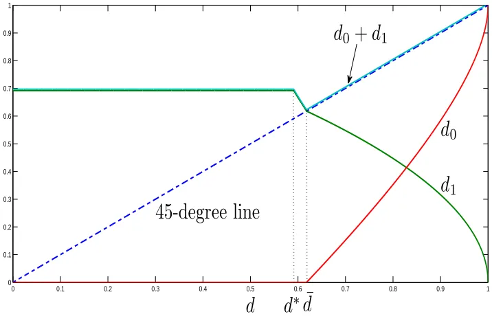
Figures 1 and 2 plot the value function and the policy functions. In Figure 2,d1 has three

segments. The flat part where d < d∗ _{corresponds to the region where the PK constraint} does not bind. The segment between d∗ _{and d}¯_{is defined by d}

1(d) =g(d) = 1−_dd; the last

segment for d > d¯is described by the policies d0 >0 and d1 >0 in (8) and (9), that is

d0 =d−

√

1₋d and d1 =

√ 1₋d.

4

Interpreting the Optimal Contract with Sharing

The previous section defines sharing to be the case where both the current and past

innovator are promised some time selling the leading-edge product; the optimal contract

employs such sharing, from (at the latest) the second innovation onward. We describe

here several interpretations of such a policy.

One interpretation of the optimal contract is as the design of an optimal policy for

patents. We see, on the one hand, that some ideas would not be allowed to profit at all;

0 0.1 0.2 0.3 0.4 0.5 0.6 0.7 0.8 0.9 1 0

0.05 0.1 0.15 0.2 0.25 0.3 0.35 0.4 0.45

d

V

(d)

Figure 1: Value function with uniform density.

0 0.1 0.2 0.3 0.4 0.5 0.6 0.7 0.8 0.9 1 0

0.1 0.2 0.3 0.4 0.5 0.6 0.7 0.8 0.9 1

45-degree line

d

d

d

+

d

d

_d

¯

d

We interpret this as being unpatentable, although our mechanism design approach

im-plies that this decision is made completely by the innovator and is not adjudicated by the

planner; the planner simply sorts out what he seeks to be unpatentable by a sufficiently

high patent fee.

On the other hand, innovations that are allowed to generate profits for the innovator

(i.e., patents issued) share with prior patents. In practice, this could occur in several

ways. For instance, when a new patent infringes on an old one, the two parties must

come to a licensing agreement. Alternatively, if infringement is not clear, the firms could

potentially engage in litigation. We argue that both outcomes can be interpreted as part

of the optimal contract with sharing.

One preset rule that allocates rights with sharing is a lottery. Suppose there is one

incumbent with a promise, d. When sharing is called for, the new innovator and the incumbent are prescribed d1 and d0, respectively. Rather than maintain that promise

for both firms, the planner could have a lottery: one of the two will be chosen to be the

new incumbent, and given a promise of d0 +d1. A lottery assigns the identity of the

new incumbent, with, for instance, the new innovator replacing the old incumbent with

probability d1/(d0 +d1). Because the innovators are risk neutral, this lottery version

of sharing implements the same allocation. In the tradition of the literature on weak

patent rights, a natural interpretation of probabilistic protection is as litigation. Here

the policy uses litigation as a method of allocating profits to different contributors; the

odds of a firm winning the litigation is tied to its share of the duration promise offered

to the two innovators under the optimal policy.

Alternatively, one can interpret sharing as coming through licensing contracts under

the circumstance where later patents infringe on early ones. One can interpret the

licensing rules as part of the social planner’s patent policy, or as a set of licensing

agreements arranged ex ante among the potential innovators; that is, the patent policy

offers a right of exclusion to all the rights holders who have a share of the profits, and the

rights holders have agreed to a preset sharing rule at time zero that maximizes expected

surplus of all potential innovators.

patents that have arrived. It is similar to standard notions of a patent pool in the sense

that many innovators have jointly contributed to the research line, and as such, they

would share in the profits of their joint effort. Here, however, the pool is ever growing as

a result of the ever-improving nature of the product. New innovators may join the pool

for a fee; in exchange they receive a share of pool profits. Whenever a new innovator

joins the pool, then, all the existing innovators’ shares drop to make room.11

In the setup we have used, the existing innovators would never want to exclude a

new innovator willing to pay the entry fee, even if they weren’t obligated to by the

commitment of the contract. To see this, notice that the marginal innovator c = d1

makes zero profit from joining the pool and improves total pool profits by contributing

an improvement; lower cost types contribute the same and get the same share, but

make profits from their lower cost c < d1. However, if contracting could only take place

after the new improvement spent c, there would be a simple hold-up problem. One can interpret the planner’s role here as to limit this hold-up. To do so, the planner should

insist on a “non-discriminatory” policy for new pool entrants that forces the pool to

pre-specify the “fair” or “reasonable” price at which they will allow new members to

join the pool, and accept membership from anyone who wants to pay the entry fee.

This gives a new role for regulation of patent pools. Policymakers have insisted that

pools treat users of the pool’s patents in a way that is FRAND.12_{The motivation for this}

policy is that a patent pool among a fixed set of innovators is like a merger between the

members, and therefore care must be exercised to make sure that patent pools don’t have

the anticompetitive effects of mergers on the pool’s users.13 _{The model proposed here}

considers how pools should be allowed to contract with potential new members, given

11

In this alternate view of the optimal contract, one might imagine the fee is no longer collected

by the central authority and rebated to consumers, but rather collected by the pool as a fee to new

entrants. This alternate view is fine; the entry fee needs only be modified to account for not only the

profits from the share of pool sales, but also the expected return to joining the pool in terms of future

fees collected from later entrants.

12

See, for example, Lerner and Tirole (2008).

13

This idea is the basis of the model of patent pools in Lerner and Tirole (2004), where pools have

welfare consequences similar to the ones found in models of mergers, based on monopoly markup by

the fact that new members increase total profits but erode pool members’ share of the

profits. To focus on the issue of how pools form, we specifically study a case where there

are no welfare consequences of the pool’s treatment of the users of the pool’s product.

Note that policies without sharing can be implemented in a much simpler way from

the licensing or litigation interpretations. Consider the optimal policy starting from

d= ¯d. In this case the policy can be decentralized through a rule that depends only on reports of arrivals. In particular, each arrival needs only to pay an entry fee, at which

point they are given the sole right to profit; that is, a completely exclusionary patent

that infringes on nothing, and allows the holder to exclude all past innovators. The

innovator who most recently paid the fee unambiguously has all the rights.

Consider, by contrast, some initial d > d¯where there is forever d0 >0 and d1 > 0.

Here decentralization requires something other than just reports of arrivals; sharing

rules conditional on those reports are essential. We view all of these constructions as

potentially generating costs relative to cases without sharing. In the next section we

consider the extreme case, where sharing is so costly that the planner must avoid it

altogether.

5

Conflict-Free Policies

Optimal policies in Section 3 included a particular sense of potential conflict,

stem-ming from sharing between multiple rights holders promised at a given history. The

planner could avoid this sort of conflict by restricting attention to policies without

shar-ing, which, upon implementing a new innovation, ends the rights of previous rights

holders. This translates to the same model of Section 3, but under the restriction that

d0 = 0. Since avoiding conflict in this sense adds a constraint, doing so always comes

at a cost. In this section we will ask two questions: First, what are the implications

of following such a policy? And second, what can we say about the costs imposed by

5.1

Optimal Policies

When d0 = 0 is imposed in (5), the Bellman equation becomes

W(d) = max

˜ d

˜

dλR(g( ˜d)) + (1₋d˜)W(g( ˜d))

s.t. d_≤d,˜ (14)

where W(_·) denotes the conflict-free value function.

Lemma 2 W(_·) is weakly decreasing and concave in d. dλR˜ (g( ˜d)) + (1₋d˜)W(g( ˜d)) is strictly concave in d˜.

Let d∗∗ _{be the unique maximizer of ˜dλR(g( ˜d)) + (1−d}˜_{)W(g( ˜d)). Then W(·) is flat}

below d∗∗_{, but strictly decreasing above d}∗∗_{. In other words, PK constraint (14) binds}

if and only if d > d∗∗_{. When it binds, the choice of d}

1 is pinned down by the constraint

˜

d=d, that is,d1 =g(d). When the PK constraint doesn’t bind, ˜d=d∗∗andd1 =g(d∗∗).

To summarize, the optimal policy is ˜d(d) = max(d, d∗∗_{), or equivalently}

d1(d) = min(g(d), g(d∗∗)).

The evolution of duration promises critically depends on d∗∗_{. As we will show, d}∗∗ _is

either equal to or below ¯d, with quite different dynamics of promises under the two cases.

Proposition 4 (i) (1 +λ)−1 _{< d}∗∗_≤d¯_.

(ii) d∗∗_{= ¯d if and only if F( ¯d)≥df}¯ _{( ¯d).}

If the density function is weakly decreasing, then d∗∗ _{= ¯d; if the density function is}

strictly increasing, then d∗∗ _<d¯_.

The condition ford∗∗_{= ¯dis that f( ¯d) is bounded above by F( ¯d) ¯d}−1_{. To understand}

why the density cannot be too large in this case, consider the optimal path of duration

promises. Denote the duration promise of thetth implemented idea asdt. Whend∗∗= ¯d,

the optimal path is perfectly smoothed, i.e., dt = ¯d for all t. Suppose we deviate and

increase d1 from ¯d to ¯d+ǫ. For simplicity, assume that this deviation does not affect dt

0 0.1 0.2 0.3 0.4 0.5 0.6 0.7 0.8 0.9 1 0

0.1 0.2 0.3 0.4 0.5 0.6 0.7 0.8 0.9 1

d

45-degree line

d

_{= ¯}

_d

d

(

d

)

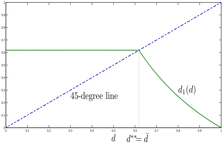
Figure 3: Conflict-free policy function with uniform density.

d2 below ¯d. Hence the benefit of a higherd1 must be weighted against the cost of a lower

d2. The cost will dominate the benefit when g(d1) is sensitive in d1. The derivative of

g(_·) is proportional to the reciprocal of the density. Hence a lower density at ¯d implies a more sensitive g(_·), which further implies that cost dominates benefit and d1 = ¯d is

optimal.

5.2

Dynamics without Sharing

When d∗∗_{= ¯d, the dynamics of duration promises are simple: if d≤d}¯_{, then d} 1 = ¯d;

otherwise if d >d¯, then d1 <d¯and d2 = ¯d. Hence we have

Corollary 3 If d∗∗ _{= ¯d, then the state variable reaches d}¯_{in at most two} implementa-tions.

Figure 3 plots the conflict-free policy function with uniform density function. It has

When d∗∗ _{< d}¯_{, the distinctive feature of the dynamics of duration promises is that}

they cycle. This is the clear sense in which a conflict-free policy always has more variable

technological progress, which we discuss in more detail below.

Proposition 5 If d∗∗ _{< d}¯_{, then either the promises to all odd implementations or all} even implementations are above d¯. Without loss of generality, suppose dt≥d¯for all odd

t. Then there exists a d_∞≥d¯such that limt→∞d2t+1 =d∞ and limt→∞d2t =g(d∞).

When d∗∗_<d¯_{, the states fluctuate around ¯dbecause ifd}

t >d¯, then dt+1 =g(dt)<d¯.

This further implies that dt+2 = min(g(dt+1), g(d∗∗)) > d¯, as both g(dt+1) and g(d∗∗)

are above ¯d. Intuitively, when the current patent protection is large, the planner cannot implement many innovations, and therefore offers a small reward to potential innovators.

Once an innovator accepts the reward, the planner no longer has to deal with such a large

patent in place, and therefore can promise more generous duration to the subsequent

innovation. This generous duration promise brings the situation back to a high level of

protection.

The two-period cycle in Proposition 5 can either be forever fluctuating (i.e., d_∞>d¯

and g(d_∞) < d¯) or converging to ¯d (i.e., d_∞ = g(d_∞) = ¯d). Figures 4 and 5 plot two dynamics of duration promises starting withd1 = 0.76. We provide sufficient conditions

for the two cases.

Proposition 6 Suppose d∗∗_<d¯_{and the initial duration promise d6= ¯d.}

(i) If g(g(c))> c for all c_∈( ¯d,1], then d_∞=g(d∗∗_).

(ii) If f(c)_≤λ−1 _{for all c∈[0,1], then g(g(c))> c for all c∈( ¯d,1].}

Proposition 7 Let b _∈( ¯d,1) be the unique solution of

Z b

0

(b₋c)f(c)dc+ (b₋1)λ−1₋R h (1₋b)λ−1

= 0. (15)

(i) If g(g(c))< c for all c_∈( ¯d, b], then d_∞ = ¯d.

(ii) If f(c) = αcα−1 _{and α is sufficiently large, then g(g(c))< c for all c}

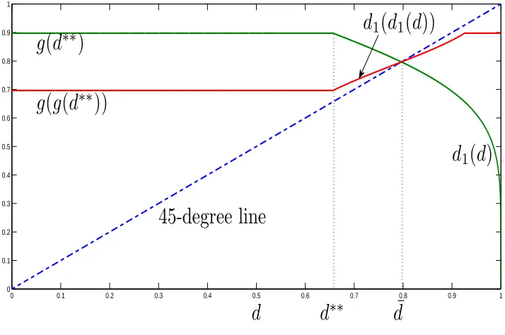
We end this section with numerical examples with power function density.

Example 2 (Power function density) Suppose that the density f(c) = αcα−1 _for

α > 1 and λ = 1. Figure 6 plots the policy function when α = 3: in a neighborhood of ¯

d, d1(d1(·)) is steeper than the 45-degree line and cycles are amplified over time. The

sufficient condition in Proposition 6 is satisfied and the cycle lasts forever. However,

when α is sufficiently large, the sufficient condition in Proposition 7 is satisfied and the states converge to d¯. Figure 7 plots the policy function when α = 6: in contrast to that in Figure 6, d1(d1(·)) is flatter than the 45-degree line and cycles disappear in the long

run.

6

Discussion

6.1

Comparison of Technological Progress With and Without

Sharing

Although welfare must be (weakly) lower without sharing, the impact on the rate of

innovations is somewhat more complicated. First, we consider the case of d∗∗ _{= ¯d; in}

that case, there are no cycles in the conflict-free policy.

6.1.1 The Case of d∗∗ _{= ¯d}

For any given d, the rate of innovation is weakly higher with sharing; it is strictly higher everywhere except ¯d.

Corollary 4 d1(d) is weakly higher with sharing, and strictly ifd 6= ¯d.

This does not, however, imply that the long-run rate of progress is higher with

sharing; the evolution of dt is endogenous, and since the planner with access to sharing

is giving out more promises from any initial starting d, that leads to more constraints later on. Define dss(d) to be the steady state value of duration starting from d; in both

1 2 3 4 5 6 7 8 9 10 0.65

0.7 0.75 0.8 0.85

Number of implemented ideas

d

Figure 4: Perpetual fluctuation with power density f(c) = 3c2_.

1 2 3 4 5 6 7 8 9 10

0.76 0.77 0.78 0.79 0.8 0.81 0.82 0.83 0.84

Number of implemented ideas

d

0 0.1 0.2 0.3 0.4 0.5 0.6 0.7 0.8 0.9 1 0

0.1 0.2 0.3 0.4 0.5 0.6 0.7 0.8 0.9 1

d

45-degree line

g

(

d

₎

g

(

g

(

d

₎₎

¯

d

d

d

(

d

)

d

(

d

(

d

))

Figure 6: Policy function with power density f(c) = 3c2_.

0 0.1 0.2 0.3 0.4 0.5 0.6 0.7 0.8 0.9 1 0

0.1 0.2 0.3 0.4 0.5 0.6 0.7 0.8 0.9 1

d

45-degree line

g

(

d

₎

g

(

g

(

d

₎₎

¯

d

d

d

(

d

)

d

(

d

(

d

))

without sharing, and greater than ¯d with sharing so long as initial duration is not ¯d, we have

Corollary 5 d1(dss(d)) is weakly higher without sharing, and strictly if d6= ¯d.

For any starting duration where sharing and non-sharing differ (d ₆= ¯d), the same pattern emerges: sharing leads to faster progress initially, but, as a result of the higher

promises given out, the long-run progress is slower. The intuition is that, with sharing,

the planner perfectly smooths the duration at his disposal, offering equal duration to

every arrival. The planner prefers smooth paths because they don’t bypass low-cost

ideas at some points in time and implement higher-cost ideas later on. Without sharing,

the planner can never achieve this smoothing if his promise rises above ¯d. To deliver the large duration promise, only the lowest-cost follow-up innovations are allowed; that

is, d1 is very low. Once a follow-up innovation is implemented, however, we implement

further follow-ups at a constant rate λF( ¯d). The welfare benefits of sharing come from the benefits of smoothing: smoother progress under sharing more efficiently implements

ideas by not bypassing low-cost ideas when d1 is low.

6.1.2 The Case of d∗∗ _<d¯

When d∗∗ _{< d}¯_{, sharing clearly leads to more variable growth, since promises cycle.}

In terms of the short-run rate of progress, if d _≥ d¯, then d1(d) is higher with sharing,

and therefore conflict-free policies have slower technological progress. If d <d¯, whether

d1(d) is higher with sharing depends on whether d∗ < d∗∗.14

The comparison of long-run growth with and without sharing could go either way in

this case. To see why the lack of sharing might lead to slower long-run growth, consider

example 2, where the contract enters a perpetual cycle for all d > d¯. The long-run growth rate fluctuates between λF(g(d_∞)) and λF(g(g(d_∞))), and the average may be lower than λF( ¯d). If the initial promise is only slightly above ¯d, the growth rate of the sharing contract will be arbitrarily close to λF( ¯d), and dominate the average growth rate without sharing.

14

In the next subsection, we further the point about sharing and convexification by

describing an environment where the initial duration promise may be large, due to the

special costs that might come with being a market pioneer. In that environment, the

feature that non-sharing leads to faster long-run growth is restored, as the growth rate

of the sharing contract is sufficiently low.

6.2

Application: Ironclad Patents and Rewarding a Market

Pioneer

A fundamental force in the model is that rewards for innovation come through market

profits, and those profits are limited. As such, it is natural to consider how the planner

might respond to a special innovation that is essential to the development of the product

but requires extra rewards in order to be implemented, such as a pioneering innovation

that begins the process. We treat the required duration promise for the initial innovation

as not stemming from the cost function or profitability described above. We imagine

that the initial duration promise reflects the particulars of the original innovation; for

instance, if the innovation were either not initially fully commercialized or very costly,

the initial duration promise required would be very great.15 _{The main goal is to show}

that this can map neatly into an initial duration promise anywhere in the unit interval,

at which point one can use the analysis of the prior sections to assess how the planner

proceeds with and without sharing.

We focus on the case where the promise d to the pioneer satisfies g(g(d)) = 1. The promise is large in the sense that the PK constraint binds with and without sharing. If

sharing is possible, a high promise to the pioneer is realized by continuous sharing: the

rate of implemented arrivals is constant, and that rate is lower the larger is the pioneer’s

promise. A larger promise translates to a greater share of future profits for the pioneer,

and therefore only lower-cost improvements are profitable.

If sharing is impossible, an initial large promise d leads to an initial rate of progress lower than with sharing, as the high duration promise to the pioneer can only be realized

15

through severe exclusion restrictions. One can think of such a patent as ironclad in the

sense that it keeps many potential entrants out of the market. However, once an idea

whose cost is lower than g(d) arrives, it will be implemented and break the ironclad patent. In other words, the pioneer’s rights are stronger without sharing, but are fully

gone sooner. Since the duration promise to the low-cost idea,g(d), is less than (1 +λ)−1_,

PK constraint becomes slack immediately after the implementation of the low-cost idea.

The continuation contract starts afresh as if the planner is not committed to any duration

promise. As we mentioned, sharing leads to smooth progress due to constant sharing with

the pioneer, while avoiding conflict forces the planner to temporarily reduce progress,

but allows progress to rise later on. This leads to a less smooth path of progress without

sharing, which is costly to the planner.

7

Conclusion

In this paper we have constructed optimal allocations for a sequence of innovators

who, due to moral hazard, must be rewarded with profit-making opportunities. We

have shown that the optimal allocations involve sharing so that more than one firm get

a share of future profits. We interpret this sharing as patents that infringe on prior

art, together with licensing. We show how the licensing contract can be interpreted as

an ever-growing patent pool and provide theoretical foundations for observed practices

like patentability requirements and infringement, as well as weak patent rights. By

constructing allocations that do not allow the planner to use shared rewards, we can

explore the role of licensing contracts in technological progress. Sharing contracts lead

to smoother progress. They also lead to faster progress initially.

We focus on the extreme case where the planner either uses sharing, or the cost of

sharing is infinite. A natural topic for future research is to see what degree of sharing the

planner would choose if faced with a finite cost of assigning shared rights. The trade-off

in making that decision is highlighted by the analysis here: Sharing is valuable as a

Appendix

Proof of Proposition 1: The concavity of the value function will be verified in Propositions 2, 3 and Lemma 1 of this paper. Let µ(d) be the Lagrange multiplier on the PK constraint (1). The first-order conditions for ˆd and ˙d are

λ(1₋F(d1))V′( ˆd) +λ(1−F(d1))µ(d) = 0,

V′_{(d) +µ(d) = 0,}

which imply that V′_{( ˆd) =V}′_{(d), and hence ˆd=d.}

The envelope condition is

−(1 +λ)V′_{(d) +V}′′_{(d) ˙d−(1 +λ)µ(d) = 0,}

which implies that ˙d= 0 because V′_{(d) +µ(d) = 0.}

Proof of Proposition 2: To show the monotonicity and concavity of Vr(·), it

is equivalent to show that V′

r(d) is negative and decreasing in d. Recall that d1(d) =

h((1₋d)λ−1_{). Then V}′

r(d) =λ(R(d1(d)))′ is

−R′(d1)h′((1−d)λ−1) = −

R′_(d 1)

(F(d1)d1)′

= −(1−d1)

d1+F(d1)/f(d1)

,

which is negative and increasing in d1 under assumption 1. As d1 decreases in d, Vr′(d)

is decreasing in d.

Next we verify the Bellman equation (6). Pick a feasible ( ˜d0,d˜1), and let ˜d2 ≡

h1−( ˜d1+ ˜d0)

λ

. Then ˜d0 = 1−d˜1−λd˜2F( ˜d2), and the PK constraint, after simplification,

becomes

1_≥ d+ 1 1 +λF( ˜d1)

λF( ˜d1) ˜d1+

λF( ˜d1)

1 +λF( ˜d1)

λF( ˜d2) ˜d2. (16)

The objective on the right side of (6) is

λR( ˜d1)

1 +λF( ˜d1)

+ λF( ˜d1) 1 +λF( ˜d1)

V( ˜d1+ ˜d0) =

λR( ˜d1)

1 +λF( ˜d1)

+ λF( ˜d1) 1 +λF( ˜d1)

λR( ˜d2)

= λR(h(˜x1)) 1 +λF( ˜d1)

+ λF( ˜d1) 1 +λF( ˜d1)

λR(h(˜x2)),

where ˜xi = ˜diF( ˜di), i= 1,2. Because R(h(·)) is concave,

λR(h(˜x1))

1 +λF( ˜d1)

+ λF( ˜d1) 1 +λF( ˜d1)

λR(h(˜x2)) ≤ λR h

1 1 +λF( ˜d1)

˜

x1+

λF( ˜d1)

1 +λF( ˜d1)

˜

x2

!!

≤ λR h (1₋d)λ−1

=Vr(d),

Proof of Lemma 1: To show that the objective in (11) is concave, note that Lemma A.1 and Lemma A.2 show that both dR(g( ˜d)) and (1₋d)Vr(g( ˜d)) are concave in ˜d.

To show that d∗ _<d¯_{, it is sufficient to verify that}

˜

dλR(g( ˜d)) + (1₋d˜)Vr(g( ˜d))

′

|_{d= ¯}˜ _d<0.

Because

V′

r( ¯d) =−

(1₋d¯)f( ¯d)

F( ¯d) +f( ¯d) ¯d, g

′_{( ¯d) =−} 1 +λF( ¯d)

2

λf( ¯d) , Vr( ¯d) =λR( ¯d), it follows from Lemma A.3 that

˜

dλR(g( ˜d)) + (1₋d˜)Vr(g( ˜d))

′

|_{d= ¯}˜ _d

= ₋1−_¯d¯

d + (1−d¯)

(1₋d¯)f( ¯d)

F( ¯d) +f( ¯d) ¯d

1 +λF( ¯d)2

λf( ¯d) = ₋λF( ¯d) + λ(F( ¯d))

2

F( ¯d) +f( ¯d) ¯d

= ₋ λF( ¯d)f( ¯d) ¯d

F( ¯d) +f( ¯d) ¯d =−

(1₋d¯)f( ¯d)

F( ¯d) +f( ¯d) ¯d =V

′

r( ¯d)<0.

Proof of Proposition 3: The concavity of V(_·) is shown in the proof of Lemma 1. To see that V′_{(·) is continuous at ¯d, recall from the proof of Lemma 1 that}

lim

d↑d¯V

′_{(d) =−} (1−d¯)f( ¯d)

F( ¯d) +f( ¯d) ¯d =V

′

r( ¯d) = lim d↓d¯V

′

r(d) = lim d↓d¯V

′_(d).

Finally we verify the Bellman equation when d <d¯,

V(d) = max

d0,d˜ ˜

dλR(g( ˜d)) + (1₋d˜)Vr

g( ˜d) +d0

s.t. d_≤d˜+ (1₋d˜)d0.

Pick a feasible (d0,d˜) such that d0 > 0. We show that V(d) ≥ dλR˜ (g( ˜d)) + (1 −

˜

d)Vr(g( ˜d) +d0). First, (d0,d˜) cannot be optimal if ˜d ≥d¯. If ˜d≥d¯, then

˜

dλR(g( ˜d)) + (1₋d˜)Vr

g( ˜d) +d0

< dλR˜ (g( ˜d)) + (1₋d˜)Vr(g( ˜d))

≤ dλR¯ (g( ¯d)) + (1₋d¯)Vr(g( ¯d))