Inferences under a Class of Finite Mixture Distributions Based on Generalized Order Statistics

(1)

Inferences under a Class of Finite Mixture Distributions

Based on Generalized Order Statistics

Abd EL-Baset A. Ahmad1, Areej M. AL-Zaydi2 1_{Department of Mathematics, Assiut University, Assiut, Egypt}

2_{Department of Mathematics, Taif University, Taif, KSA}

Email: [email protected], [email protected] Received May 1, 2012; revised January 2, 2013; accepted January 19, 2013

Copyright © 2013 Abd EL-Baset A. Ahmad, Areej M. AL-Zaydi. This is an open access article distributed under the Creative Com-mons Attribution License, which permits unrestricted use, distribution, and reproduction in any medium, provided the original work is properly cited.

ABSTRACT

The main purpose of this paper is to obtain estimates of parameters, reliability and hazard rate functions of a heteroge-neous population represented by finite mixture of two general components. The doubly Type II censoring of generalized order statistics scheme is used. Maximum likelihood and Bayes methods of estimation are used for this purpose. The two methods of estimation are compared via a Monte Carlo Simulation study.

Keywords: Generalized Order Statistics; Bayes Estimation; Heterogeneous Population; Monte Carlo Integration; Monte Carlo Simulation

1. Introduction

Let the random variable (rv) T follow a class including

some known lifetime models, its cumulative distribution function (CDF) is given by

 

1 exp

 

, 0,



0 ,

F t   _ t _ t  





(1)

and its probability density function (PDF) is given by

 

exp

 

, 0,



0 ,



f t  t _ t _ t  (2)

where is the derivative of with respect to t

and

 

t



 

t

 

t



 

t;

   is a nonnegative continuous function of t and  may be a vector of parameters, such

that

 

t 0 as t0 and 

 

t   as t .

The reliability function (RF) and hazard rate function (HRF) are given, respectively, by

 

exp

 

,

R t   t  (3)

 

,

H t  t (4)

where

 

.

   

.

H  f R . .

Bayesian inferences based on finite mixture distribution have been discussed by several authors. Bayesian estima-tion of the mixing parameter, mean and reliability func-tion of a mixture of two exponential lifetime distribufunc-tions based on right censored samples considered by [1,2]

es-timated the survival and hazard functions of a finite mix-ture of two Gompertz components by using type I and type II censored samples, using the maximum likelihood (ML) and Bayes methods. Based on type I censored sam-ples from a finite mixture of two truncated type I general-ized logistic components, [3] computed the Bayes esti-mates of parameters, reliability and hazard rate functions. [4] considered estimation for the mixed exponential dis-tribution based on record statistics. [5] considered Bayes inference under a finite mixture of two compound Gompertz components model. [6] studied some properties of the mixture of two inverse Weibull distributions and obtained the estimates of the unknown parameters via the EM Algorithm.

[7] introduced the generalized order statistics (gos’s). Ordinary order statistics, ordinary record values and se-quential order statistics are, among others, special cases of gos’s. The gos’s have been considered extensively by many authors, among others, they are [8-20].

Mixtures of distributions arise frequently in life testing, reliability, biological and physical sciences. Some of the most important references that discussed different types of mixtures of distributions are a monograph by [21-23].

The PDF, CDF, RF and HRF of a finite mixture of two components of the class under study are given, respec-tively,

 

1 1

 

2 2





,

(2)

 

1 1

 

2 2





,

F t  p F t p F t (6)

 

1 1

 

2 2



,

R t  p R t p R t



(7)

 

   

,

H t  f t R t (8)

where, for j1, 2, the mixing proportions pj

 

are such

that 0 pj1,p1p21 and fj

 

t ,Fj t ,Rj

 

t are given from (1), (2), (3) after using j and j

 

t in-stead of  and 

 

t .

The property of identifiability is an important consid-eration on estimating the parameters in a mixture of dis-tributions. Also, testing hypothesis, classification of ran-dom variables, can be meaning fully discussed only if the class of all finite mixtures is identifiable. Idenifiability of mixtures has been discussed by several authors, including [24-26].

Our aim of this paper is the estimation of the parame-ters and functions of these parameparame-ters of a class of finite mixture distributions based on doubly Type II censoring gos’s using ML and Bayes methods. Illustrative example of Gompertz distribution is given and compared with the results obtained by previous researchers.

2. Maximum Likelihood Estimation

Let

; , , , 1; , , , , ; , , ,1 ,

s n m k s n m k r n m k

T T T   s r n k0,

be the (r - s) gos’s drawn from a mixture of two

compo-nents of the class (2). Based on this doubly censored sample, the likelihood function can be written [27] as

 





 

_{ }

  

 

1 1 1 1 1 0 1 2 , 1

ln , 1,

r m

r

i i r

i s s m s s s s k r

r s i s i

c R t f t R t

L t R t m

c R t R t H t m

             _ _ _ _       _ _ _  _ _     ,    _ _   







    (9) where t



t_s, , t_r



, Θ,  is the parameter space, and



 













 

_{ }

1 1 1

1 1 2

1 1

( 1) ( 1)

, ,

1 !

1 1 !

, 1 1 1 . s s r s r

r j j r

s

C k

c c

s

m s

C k n r

s               , r m     _               _ _ _   _



  _

For definition and various distributional properties of gos’s, see [7, 28].

The likelihood function (9) and maximum likelihood estimates (MLE’s) can be obtained by using (1) and (5) in two cases, regarding to m value, as follows.

2.1 MLE’s When m 1

In this case, substituting (1), (5) in (9), the likelihood function takes the form

 



 

_{ }

  

1

1 1 1 2 2

1 1 2 2

1 ₁ ₁

1 1 2 2 0 . r r _m i i i s i i r r s s m s s s

L c p R t p R t

p f t p f t

p R t p R t

      _{ } _   _ _  _ _  _    _  _ _  _    _  _





   t (10)

Take the logarithm of (10), we have

 

_{ }

  

1 1 1 2 2

1 1 2 2 1 1 1 2 2

1 ₁ ₁

1 1 2 2 0

ln ln ln

ln ln ln , r i i i s r

i i r r

i s

s _s _m

s

s s

L c m p R t p R t

r

p f t p f t p R t p R t

p R t p R t

        _{ } _       _  _    _  _ _  _  _ _    _  _   



t     (11) where p1 p, p2 1 p.

Differentiating (11) with respect to the parameters , j

p and j (involved in ) and equating to zero gives the following likelihood equations

 

   

 

   

 

   

 

   

1 *

* * 0

1 1 0 * * 1 1 * 0 1 0 * * 0,

0, 1, 2, s

s s

r r

i i r r s

i s i s

s

r r

j j i j i j j i j i

i s i s

j

r j j r j r

s

s j j s j s

s

r

j i

j j j i j j

i s

j j

t t

m t t t

p

t

m p t t p t t

p t t

t p t t

j t

t

m p t p t

                                               _{ } _        _{ } _  



          

_{   }

   

 

   

 

* 1 1 * 0 1 0

0, 1, 2 r

i j i i s

j r

r j j j r

j

s

j s

s j j j s

j s s t t p t t

t p t

j t                                          _  _  _         _  



    (12) w

(3)

 

_{ }

 

_{ }

 

_{ }

 

_{ }

 

_{ }

 

_{ }

_

_

1 2 * 1 2 * * 1 1 , ,

, , , , 1

j i j i i i

j i j i j i j i

j j i j j i

j i j i s

i i

i j i j i s s

i i i

t t f t f t

t t t t

t f t

f t R t

R t R t

t t t t R t s

R t f t R t

                               



, 1 m     _    _         _          _{ }     (13)

The solution of the five nonlinear likelihood Equa-tions (12) using numerical method, yields the MLE’s

1 2 1

ˆ ˆ ˆ ˆ, , ,

p   and ˆ₂.

2.2. MLE’s When m 1

The likelihood function takes the form

 



 



1 _{1 1}

 

_{ }

_{2 2}

 

_{ }

2 1 1 2 2 1 1 2 2

1 1 2 2

ln s r .

k i

r r s s

i s i i

p f t p f t

L c p R t p R t p R t p R t

p R t p R t

   i         _  _  _  _      



t (14)

So, from (14)

 

  





 



 





1 1 2 2 1 1 2 2

ln 1 ln ln

ln ln .

r r s

r

i i i i

i s

k p R t p R t s p R t p R t

p f t p f t p R t p R t

  s    _  _  _  _     



_  _ _  _  (15)

Differentiating (15) with respect to the parameters ,pj and j and equating to zero gives the following like-lihood equations

  

    



 



    



     



   



     

   

* * * * * * * * * 1 0, 1

0, 1, 2,

1 r

r s s i i

i s

r

j j r j r j j s j s s j j i j i j j i j i

i s j

j r j s j i

j j j r j j j s s j j i j i j j j i

i

j j j j

k t s t t t t

p

kp t t s p t t t p t t p t t

j

t t

kp t s p t t p t t p t

                                  _ _{ } _ _ _   _{ } _{ } _ _          _{ } _{ } _ _        _  _



  

0, 1, 2

r s j   * t               



(16)

where where Ω is the hyperparameter space.

 

1

_{ }

.

ln i

i

t

R t

  (17) 3.1. Bayes Estimates When m 1

It follows, from (10) and (18), that the posterior density function is given by

The solution of the five nonlinear likelihood Equa-tions (16) using numerical method, yields the MLE’s

1 2 1

ˆ ˆ ˆ ˆ, , ,

p   and ˆ₂.

 

_{ }

1 * 1

1 1 2 2 1 1 2 2

1 1 2 2 1

1 1 2 2 0

π ; exp ;

r r

m

i i i

i s

r r

s s

A C D

p R t p R t p f t p f t

p R t p R t

             _ _ i  _ _{ } _ _ _  _{ }  __   _  _    _  _





  t (19)

3. Bayes Estimation

In this section, Bayesian estimation for the parameters of a class of finite mixture distributions is considered under squared error and Linex (Linear-Exponential) loss functions.

We shall use the conjugate prior density, that was

suggested by [29], in the following form where

 

1

1 π ;

A L



 



1 2 1 2



π ; ; exp ;

, , , , , , C D p              _    d .    

 _

_

_t ₍₂₀₎

, 

(4)

squared error and Linex loss functions is given, respec-tively, by

 





 

*

 

ˆBS π d ,

u E u u



   

 t 

_

t (21)

 





  *

_{ }

1

ˆ ln e

1_ln _e _π _d _,

au BL au u E a a           _ _    _

_

t

t _

(22)

where the integral is taken over the five dimensional space and a0.

To compute the integral, we can use the Monte Carlo Integration (MCI) method in the form

   

 

1 1 ˆ , M j j j BS M j j u L u L      



t t (23)

 

_{ }

 

1 1 e 1

ˆ ln ,

j M _au j j BL M j j L u a L                   



t t  (24)

where j,_j_1, 2, ,_ _M



is generated from the PDF



π  ; , for more details see [30].

Under squared error and Linex loss functions, we can obtain the Bayes estimator of the parameter p, by

generating



, 1, 2, 1, 2



1, 2, ,

j j j j j

p     j  M p

from the prior (18) and setting in (23) and (24). The Bayes estimates of

 

u  

1, ,2 1

   and 2 can be similarly computed.

3.2. Bayes Estimates When m 1

The posterior density function can be obtained from (14) and (18), as

 





 

* 2

1 1 2 2

1 1 1 2 2

1 1 2 2

π ; exp ;

ln k r r s s s r i i

i s i i

A C D

p R t p R t

p f t p f t

p R t p R t

        _ _ _  _    _  _           



t (25) where

 

1

2 π( ; ) d .

A L

    

 _



t (26)

Under squared error and Linex loss functions, we can obtain the Bayes estimator of the parameter p, by

generating



, 1, 2, 1, 2



1, 2, ,

j j j j j

p     j  M

p

from the prior (18) and setting in (23) and (24). The Bayes estimates of

 

u  

1, ,2 1

   and 2 can be similarly computed.

4. Example

4.1. Gompertz Components

4.1.1. Maximum Likelihood Estimation Suppose that, for j1, 2 and t0,_j1,

 

1 e jt 1

j j t       _  _ so

 

e jt

j t

  

th

.

In this case, the j subpopulation is Gompertz

distribution with parameter  j 0.

For m 1 by substituting _j

 

t and j

 

t in (12), we have the following nonlinear equations

 

   

 

   

 

   

 

* * 1 1 * 0 1 0 * * * 1 1 * 0 1 0 0, ,

0, 1, 2 r

i i s r

i r r

i s s s s s s r

j j i j i i s

j

r

j j i j i i s

r j j r j r

s

s j j s j s

s s m t p t t t t t

m p t t

p t t

t p t t

j t                                   _    _    _           _{ }    _       _       _   



          (27)

where, for j1, 2

 





 





* 2 1

1 e 1 ,

, ,

1 ₁ _{1 e}

j

j i t

j i

j

j i i j i

t

j i j i

j

t

t t t

t t              _     _      _    (28) 1 ˆ ˆ,

p and ˆ₂ are the solution of the above nonlinear

equations.

Also, for m 1 substituting _j

 

t and _j

 

t in

(13), (16) and (17), we have the following nonlinear equa 

(5)

  

    



 



    



     



   



* * * * * * * 1 0, , 1 0 r

r s s i i

i s

r

j j r j r j j s j s s j j i j i j j i j i

i s j

k t s t t t t

p

kp t t s p t t t p t t p t t j

                  _ _{ } _ _ _ 

, 1, 2

  _   _           _





 (29)

1 ˆ ˆ,

p and ˆ₂ and k1 in (10),



_r r 1 ,



0

m

are the solution of the above nonlinear

ases

r statistics

If we put equations.

Special c   n

1) Upper orde the likelihood function takes the form

 

1  

_{ }

1

1 1 1 2 2 1 1 2 2 1 1 2 2

0

.

r s

s

n r _s

i i r r s s

i s

L  c p f t p f t p R t p R t  p R t p R t

 _{ }       



_  __  _ 



_ _   

t  (30)

Substituting m0,k1 and r  n r 1 in (27), we have the following nonlinear equations

   

  

  

1 * s t t   

 

    



   

 

   

 

* 0 1 0 1 *

* * 0

1

0

0,

,

0, 1, 2

s s

r

i r s

i s

s

s j j s j s r

j j i j i j j r j r s

i s j

s

t n r t

p

t

t p t t

p t t n r p t t j

t            _             _                   _  _ 



          (31) here

w    s  1. The

(3

2) Upper record values

If we put k1 in (14), the likelihood

fu





1 r  

nction takes the form solution of the nonlinear likelihood equations

1) gives the MLE’s pˆ,ˆ1 and ˆ2.

 



 



1 _{1 1}

 

_{ }

_{2 2}

 

_{ }

2 1 1 2 2 1 1 2 2

1 1 2 2

ln s r i i .

r r s s

i s _i

p f t p f t

L c p R t p R t p R t p R t

p R t p R t

   i         _  _ _  _      



t (32)

Substituting k1 in (29), we have the following nonlinear equations



    

 

    



     

   

1

* *

1 r r 0,

s  t  t  t  t













1

* * *

,

1 0, 1, 2

s s i i

i s i s

r r

j j i j i j j s j s s j j i j i

i s i s

j

p

p t  t s p t  t  t p t  t j

       _ _    _   _ _{ } _ _ _ _  



_ 

 (33)

The solution of the nonlinear likelihood Equations 3

( 3) gives the MLE’s pˆ,ˆ1 and ˆ2. 4.1.2. Bayes Estimation

Let p,₁ and ₂ are independent random variables such that p~Beta b b



1, 2



and for j1, 2, j to

follow a le ponential d w

pa-rameter

ft truncated ex ensity ith

j

d



LTE d

 

_j



, as used by [2]. A joint prior

density fu ctin on is then given by

 

1 2





2

1 1

b b 

1 2

1 1

; exp j ,

j j p p d              



 (34) where 0





1 1 2 1 2

0 p 1,_j 1, b b d d, , ,  and p2 1 p1.

For m 1, the posterior density function π*

 

t then takes the form

 





 



1 1 2 2 1 1 2 2

r

m

i i i i

i s

p R t p f t p f t



 

_{ }

1 2 1 2 1 1 1 2 1 1

1 1 2 2 1 1 2 2

0 1 π exp r j b b j j s s

r r s s

p p

d

p R t

p R t p R t p R t p R t

(6)

For m = −1 the posterior density function_π*

 

_

t then takes the form

 

1 2





 



 



 

_{ }

 

_{ }

2 ₁

1 1 2 2

1 1 *

1 2 1 1 2 2 1 1 2 2

1 1 1 2 2

1

π b b exp j k ln s r i i .

r r s s

j j i s i i

p f t p f t

p p p R t p R t p R t p R t

d p R t p R t



   

 

   _  _

   

  _  _  _  _

  

  _ _









t

(36)

Under squared error and Linex loss functions, we

ca eter

generating M from th ior

(34) and set 3) and (24 e

Bayes esti

n obtain the Bayes estimator of the param by



j j j



p

e pr ). Th 1 2

, , 1, 2, ,

p   j 

ting u

 

  p in (2

mates of ₁ and ₂ can be si rly

computed. ses

1) Upper order statistics If we put

mila

Special ca

in (35),



_r   n r 1 ,



t m

and k1 0

m he

posterior density function takes the for

 

1 2





 

_{ }

2 1

1 1 *

1 2 1 1 2 2 1 1 2 2 1 1 2 2

1 i i r

j dj i s 0

1

π b b exp j r n rs s .

r s s

p p  p f t p f t p R t p R t p R t p R t 

    



  

     

 





_  __  _



 _  _

 t

(37) record values

n (36),

 

 

 

2) Upper

If we put k1 i



r 1 ,



the posterior density function takes the form

 





 



 



 

11 21 1 1 1 2 2

*

1 2 1 1 2 2 1 1 2 2

1 1 1 2 2

π b b exp j ln s i i .

r r s s

j j i s i i

p f t

p p p R t p R t p R t p R t

d p R t p R t

   

 

 _ _

   

  _  _ _  _

  

  _ _









t

(38)

Linex loss functions, we

ca he B ator of

by generating M from

prior (34) and

2  1

  r _{p f t}  

Under squared error and

n obtain t ayes estim the parameter p,

j j j



p , 1, 2



j1, 2, ,

setting u

 

 p

the

 in (23) ates of 1

and (24). Th Bayes estim  and 2 can be simila e computed.

. Simulation Study

ed error or a Linex l arlo simu

ist

in

given values of the prior parameters ndom value from the

rly

5

A comparison between ML and Bayes estimators,

un-der either a squar oss functions, is

made using a Monte C lation study in the two cases upper order stat ics and upper record values according to the follow g steps:

1) For a



b b1, 2



generate a ra



1, 2



Beta b b distribution.

p

2) For a given values of the prior parameters dj, for j1, 2, generate a random value j from the

 

j

LTE d distribution.

3) Using the generated values of p,₁ and ₂, we generate a random sample of size





fro

20,30,50

n

m a mixture of two Gomp

 

_j componen

1, 2,

j as follows:

 generate tw

ts,

o observations u u₁, ₂ from Uniform 0,1 .

 

 if u₁ p, then





1 2

1 otherwise

1 _{log 1} _{log 1}

t  u



 _  





2 2

2 log 1

t



 1 _  log 1u _.

 repeat above steps times to get a sample of si e .

4) The sample obtained in Step 3 is ordered. 5) The MLE’s of the parameters

n z

n

1 ,

p and ₂ are

obtained by solving the nonlinear y

6) U ated values of

Equations (31), b using Mathematica 6.

sing the gener p,1 and 2, we generate upper record values of size n



5,8,10



from a mixture of two Gomp

 

_j ,j1,2 components.

7) The MLE’s of the parameters p,1 and 2 are

obtained by solving the nonlinear y

usi ica 6.

8) The Bayes estimates under squared error and Linex loss functions (BES, BEL), of

Equations (33), b ng Mathemat

1

p and ₂

e-,

are computed, by using MCI form

squared deviations

s (23) and (24), r spectively.

9) The



 ˆ



2 are computed

for different samples and censoring sizes, where  stands for the parameter and ˆ its imate ( L or Bayes).

10) The above Steps (

est M

3)-(9) are repeated 1000 times.

Th (ER) m

ing the esti ions, respectively

computational (our) results were computed by e averages and the estimated risks are co - puted over the 1000 repetitions by averag -

mates and the squared deviat .

The ,

(7)

using Mathematica 6.0. In all above cases the pr r pa- io rameters chosen as b14.5,b23.2,d11.2, d22.3, which yield the generated values of p0.524855,

1 1.47589

  and 22.7255 (as the true values). The true values of R t

 

and H t

 

when 0.5, a

computed to be R

 

0.5 0.414044 and

t re

 

0.5

H 

2.80864. The value of the shape parameter a of the

Linex loss function is a2. The averages and the estimated risks (ER) are displayed in Tables 1-4. Fig-

ures 1 and 2 represent i-

mates in the case of upper order statistic

sent d risks of the estimates

ER) of the estimates o

the es

timate

timated risks of e est s. res 3 re the es

Ta erages s ( f

th Figu and 4 rep

ble 1. (Upper order statistics) Av and Estimated Risk 



p, 1, 2



for different samples

and censoring sizes.

n s r, Method pˆ ER p

 

ˆ ˆ1 ER

 

ˆ1 ˆ2 ER

 

ˆ2

ML 0.707005 (0.19356) 2.31845 (1.46886) 2.39962 (0.850168)

BL 0.616284 (0.00864557)

20 (2, 14)

BS 0.643168 (0.0141694)

1.09815 (0.14386) 1.13638 (2.52742)

1.10888 (0.136649) 1.16379 (2.44375)

ML 0.714324 2.25684 2.32837

BL 0.632902 1.022 1.12869

0.011701) (0.20618) (2.55009)

0.683938 1.02377 1.16001 30 (2, 21)

50

(2, 35) (

(

0.710 735) 2.36 59) 2.442 496)

20 (1, 14) BL 0.60 91) 1.10 21) 1.1209 4)

0.6239 4848) 1.1156 04) 1.15 91)

(0.188562) (1.18964) (0.716555)

( BS

(0.0254091) (0.204632) (2.45121)

ML 0.666667 2.17853 2.26631

(0.181185) (0.806393) (0.516371)

BL 0.547597 1.0264 1.06996

0.000574537) (0.20208) (2.74081)

BS 0.552577 1.02767 1.07139

0.000797349) (0.200941) (2.73608)

ML 467 (0.196 646 (1.641 19 (0.907

1193 (0.0059 452 (0.1388 (2.5769

BS 59 (0.0099 (0.1314 205 (2.480

n

 s r,

Method _ˆ

p ER p

 

ˆ ˆ1 ER

 

ˆ1 ˆ2 ER



ˆ2



2.20851 2.28107 ML _(0.195162)0.725016

(1.03578) (0.692991)

0 )

30 (

0.458447 1.04342 1.05501

(0.00464071 (0 87036) (

50 (1

BS 0.4644 2117) 1.043 845) 1.05 61)

20 BL (1, 20)

0.6 1.79 18) 2.45 87)

30 (1, 30) 1 1

(

0.626 6) 1.70 94) 2.490 18)

BL 0.56 1.6 3) 1.8386 8)

5

0.5884 4187) 1.935 391) 2.651 827)

BL BS

.60 07

0.630063 (0.0116613)

7509 (0.007664 1.0 1)

1.06868 (0.166023)

65 (0.16900 1.10 8)

1.10867 (2.61438)

095 (2.6392

1, 21)

ML 0.682439 2.15281 2.24968

(0.183833) (0.758847) (0.522389) BL

) .1 2.79062)

, 35)

08 (0.0040 64 (0.186 637 (2.78

ML 0.695272 1.89954 2.38476

(0.178062) (0.505669) (0.90054) 0.562142 1.6268

(0.00151982)

8 (0.0668917)

1.82389 (0.85426)

BS 0.589223 1.97985 2.83692

(0.00429) (0.360228) (0.411247)

ML 7 22)

6202 (0.00130063)

1677 (0.16 6 3

213 (0.083477

66 (0.353 167 (1.182

BL 0.55

0.585439

.64 9)

1.96737

.83 01)

2.67792 633 (0.8389

BS (0.004034) (0.352081)

1 7

0.375141)

ML 802 (0.14438 31 (0.209 75 (0.7916

3246 (0.00174849) 51 (0.079246 (0.82157

0 (1, 50)

(8)

 

R t and H t

 

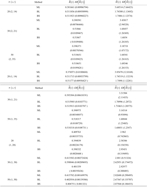
Table 2. (Upper order statistics) averages and estimated risks (ER) of the estimates of f t sample

and c es.

or differen ensoring siz

Method R tˆ  ER R t

 

ˆ  H tˆ  ER



H tˆ 



 

n s r,

ML 0.381661 (0.00906794) 3.68514 (7.66423)

BL (0.0095899 1.7430

BS (0.0096022 1.74

3.

(0.00706446) (2.94528)

BL 0.51866 1.68457

(0.0109467) (1.26369)

30 (2, 21

(0 )

50 BL

(0 )

BS

(0 ) (

ML 0.37 04) 3.85 8)

20 ( 0.5117 5799) 1.74 19)

BS 0.51 1.7 1)

0.511856 9) 8 (1.13692)

20 (2, 14)

0.511923 7) 86 (1.12574)

ML 0.388581 43017

BS 0.51867 1.6854

)

( 0.0109488) (1.26185)

ML 0.396371 3.18718

.00370546 (1.07172)

0.518651 1.68541

(2, 35) .0109425 (1.26163)

0.518651 1.68546

.0109426 1.26153)

6971 (0.01006 478 (12.016

1, 14) BL 15 (0.0095 519 (1.132

177 (0.00956825 ) 498 (1.1228

n s r, Method R tˆ  ER R t

 

ˆ  H tˆ  ER H t



ˆ 



3.31504

ML 0.3933

30 (1, 21)

(0.00348857) (0.93894)

0.518317 1.68844 50 (1, 35)

BS 0.518318 (0.0108731 ) 1.6 7)

20

(1, 20)

30 ( 0.3988 9693) 2.6295 4472)

( ) (

M 0.41 2.82 )

0.4029 9306) 2.673 707)

50 (

BS 0.40 2.87 )

84 (0.00610191)

(2.11435)

BL 0.515905 (0.0103771) 1.70996 (1.2072)

BS 0.515913 (0.0103787 ) 1.71063 (1.20575)

ML 0.398975 3.14314

BL

(0.0108729) (1.25485)

8851 (1.254

ML 0.409763 2.962

(0.00335753) (0.742865)

BL 0.394839 2.58386

(0.00226178) (0.154358)

BS 0.398332 2.95451

(0.0020448 ) (0.319495)

ML 0.413582 (0.00272424) 2.881 (0.51324)

1, 30) BL 46 (0.0020 1 (0.17

0.401559 2.92977

BS 0.00195636 0.308405)

L 5782 (0.00169979) 688 (0.290495

BL 34 (0.0013 67 (0.135

1, 50)

[image:8.595.56.539.121.735.2]

(9)

Table 3. (Upper record values) Averages and Estimated Risks (ER) of the estimates of 



p, ₁, ₂



for different sample and censoring sizes.

Method pˆ ER p

 

ˆ ˆ1 ER

 

ˆ1 ER

 

ˆ2

n s r,

2 ˆ



ML 0.631933 (0.200897) 2.67986 (2.83816) 2.89873 (1.4118)

BL 0.558404 (0.001 74504 (0.108009) 41)

5 (

BS 0.587338 (0.004 28454 (0.793391) 66)

BL 0.545122 1.99517 2.21236

(0.00066120 (0.36226) (0.334018) 8 (2, 7)

( (

10 _BL

(2, 9) (0 ( (

BS

(0 ) ( (

ML 0. 2.62 16) 2.85 7)

5 ( 0.5610 3488) 1.745 393) 1.922 007)

B

28567) 1. 1.98448 (0.5791

2, 4)

04486) 2. 3.46485 (0.7762

ML 0.564415 2.61393 3.0953

(0.193903) (2.11598) (5.09421)

6)

BS 0.574543 2.59249 3.70339

(0.00269061) (1.47151) (1.32978)

ML 0.751296 2.14647 2.93067

(0.19713) 0.632337) 23.1693)

0.553808 1.86508 2.11734

.000924086) 0.227293) 0.431788)

0.580802 2.30151 3.30646

.00320725 0.800718) 0.509574)

626796 (0.2019) 149 (2.543 242 (1.3297

1, 4) _BL 15 (0.0013 89 (0.104 57 (0.667

S 0.5882 2.27422 3.24856

 

ˆ ER p

 s r,

n Method pˆ ˆ₁ ERˆ1 ˆ2 ERˆ2

2.58457 2.9875 ML _(0.194865)0.553391

(1.69481) (2.2188)

BL 0. )

8 (

0

(0.195127) (0.627068) (5.2213)

0 21 86627 08316

(0 ( (0 )

10 (1, 9)

0.583 548) 2.24 18) 3.340 48)

5

(1, 5) ( (

8 ( 0.53871 92836) 1.896 578) 2.1096 518)

(0 ) ( (

M 0.7 7) 2.00 16) 2.6 1)

0.5473 5634) 1.824 567) 2.03 41)

10 (1, 10)

BS 0.57 2.235 433) 3.23 )

553064 (0.00100325 2.00503 (0.360188) 2.14377 (0.404423) 1, 7)

BS 0.582772 (0.0035541) 2.56838 (1.36471) 3.76664 (1.4979)

ML .737692 2.12728 2.69955

BL .5516 1. 2.

.000954124) 0.218747) .468689

BS 116 (0.00359 422 (0.6907 05 (0.6323

ML 0.69058 2.25104 2.6748

(0.195468) (1.41082) (1.11396)

BL 0.555479 1.72972 1.91339

0.00102412) (0.116361) 0.699269)

BS 0.584415 2.21588 3.26564

(0.00363311) (0.7209) (0.576103)

ML 0.671123 (0.196826) 2.28674 (1.0187) 2.85737 (4.12699)

1, 8) BL 3 (0.0003 49 (0.283 6 (0.470

0.56659 2.4252 3.41334

BS .00190609 1.13393) 0.749679)

L 89522 (0.19414 076 (0.4785 7385 (1.9245

BL 29 (0.00058 98 (0.181 864 (0.531

[image:9.595.55.543.115.738.2]

(10)

 

R t H t for different

Table 4. (Upper record values) Averages and Estimated Risks (ER) of the estimates of and sam-ple and censoring sizes.

 

ˆ

R t ER R t

 

ˆ  H tˆ  ER H t

 

ˆ 

n s r, Method

ML 0.342028 (0.0172756) 5.66515 (237.48)

BL (0.0067459 2.6813

4)

BS ( 0.0054375 3.598

4.4366

(0.0132904) (10.0859)

BL 0.312673 3.05881

(0.0125119) (0.196192)

8 (2, 7)

(0 ) (

10 BL

(2, 9) (0 ) (

B

(0 ) (

ML 0.34 86) 4.99 1)

5 ( 0.3528 0487) 2.693 445)

BS 0.36 79) 3.5 9)

0.344783 6) 9 (0.0733731)

5 (2,

0.353593 5) 21 (1.31366)

ML 0.335959

BS 0.320432 4.07878

(0.0109407 ) (2.75144)

ML 0.392196 3.26384

.00425724 1.69679)

0.349632 2.86293

.00541351 0.118538)

S 0.355924 3.46669

.00461905 0.874738)

8583 (0.01610 658 (64.601

1, 4) BL 21 (0.0053 39 (0.0650

0458 ( 0.004283 342 (1.3023

ns r,  Method R tˆ  ER R t

 

ˆ  H tˆ  ER H t



ˆ



4.31724

ML 0.338 3)

2. 8 ( 7)

(0.00356277) (1.10688)

0.350405 2.87756

(0.00522127) (

10 (1, 9)

0. 3.48 89)

5

(1, 5) (

8 ( 0.3316 0409) 2.937 037)

(

M 0.40 3.0

0.353 766) 2.840 151)

10 (

BS 0.359484 (0.0040121 ) 3.38218 (0.568505)

792 (0.01254

(6.94347)

BL 0.31614 (0.0115378) 99744 (0.157374)

1,

BS 0.323935 (0.0100044) 3.95132 (2.20381)

ML 0.394473 3.19236

BL

0.100219)

BS 356443 ( 0.00444454) 105 (0.7683

ML 0.379553 3.97702

(0.0101978) (60.4934)

BL 0.356758 2.66213

(0.00535798) 0.0984434)

BS 0.364529 3.41487

(0.00435279 ) (1.22003)

ML 0.372725 (0.0076614) 3.64809 (3.4103)

1, 8) BL 79 (0.0088 11 (0.172

0.338926 3.74408

BS 0.0076069 ) (1.62913)

L 6745 (0.00339404) 1535 (1.01302)

BL 242 (0.004 17 (0.097

[image:10.595.57.540.123.738.2]

(11)



p, ₁, ₂





[image:11.595.133.465.85.384.2]

   , R t

 

and H t

 

Figure 1. Estimated Risks (ER) of the estimates of based on doubly Type II censored

samples (s = 2).



p, 1, 2





   , R t

 

and H t

 

[image:11.595.131.467.431.714.2]

(12)

[image:12.595.130.468.85.376.2]

Figure 3. Estimated Risks (ER) of the estimates of 



p, ₁, ₂



, R t

 

and H t

 

base on doubly Type II d censored samples (s = 2).



p, ₁, ₂





   , R t

 

and H t

 

[image:12.595.126.469.422.714.2]

(13)

in the case of upper record values.

6 Concluding Remarks

1) Estimation of the parameters of the finite mixture model of two Gompertz distributions are considered from a Bayesian approach based on gos’s. A compare- son between ML and Bayes estimators, under either a squared error loss or a Linex loss, is made by using a Monte Carlo simulation study in both two cases con- sidering order statistics and upper record values cases.

2) From Tables 1 and 2, we see that in most of the considered cases, the ER’s of the estimates decrease as

n increases. In complete sample case, the Bayes esti-

mates of p,

[3] E. K. AL-Hussaini and S. F. Ateya, “Bayes Estimations under a Mixture of Truncated Type I Generalized Logistic Components Model,” Journal of Applied Statistical Sci- ence, Vol. 4 No. 2, 2005, pp. 183-208.

[4] Z. F. Jaheen, “On Record Statistics from a Mixture of Two Exponential Distributions,” Journal of Statistical Computation and Simulation, Vol. 75, No. 1, 2005, pp. 1- 11. doi:10.1080/00949650410001646924

[5] E. K. AL-Hussaini and R. A. AL-Jarallah, “Bayes Infer- ence under a Finite Mixture of Two Compound Gompertz Components Model,” Cairo University, 2006.

[6] K. S. Sultan, M. A. Ismail and A. S. Al-Moisheer, “Mix- ture of Two Inverse Weibull Distributions: Properties and Estimation,” Computational Statistics & Data Analysis, Vol. 51, No. 11, 2007, pp. 5377-5387.

doi:10.1016/j.csda.2006.09.016

1

 and HRF under Linex loss function

have the sm st ER’s as compared with their corresponding esti tes under squared error loss function or MLE’, wh R’s of the Bayes estimates of

alle ma

ile the E 2

he s, the on have

on or ro-

[7] U. Kamps, “A Concept of Generalized Order Statistics,” Journal of Statistical Planning and Inference, Vol. 48, No. 1, 1995, pp. 1-23. doi:10.1016/0378-3758(94)00147-N and RF under squared error loss functions are t

smallest es ted risks. For censored sample Bayes estim of p under Linex loss functi

the smallest ER’s as compared with their correspond-ing estimates under squared error loss functi MLE’s. Whi the Bayes estimates (against the p posed prior) o

tima ates

le, f 1

[8] M. Ahsanullah, “Generalized Order Statistics from Two Parameter Uniform Distribution,” Communications in Statistics—Theory and Methods, Vol. 25, No. 10, 1996, pp. 2311-2318. doi:10.1080/03610929608831840

[9] U. Kamps and U. Gather, “Characteristic Property of Generalized Order Statistics for Exponential Distribu- tions,” Applied Mathematics (Warsaw Vol. 24, No. 4, 1997, pp. 383-391.

[10] E. Cr er a amps tations of S

and HRF under squared error

functi orrespon

n is in

Also, we not he MLE’s of

loss

creased. on have the sm

e th

),

allest ER’s as compared with their ding estimates. It is observed that MLE’s for

c am nd U. K , “Relations for Expec

Functions of Generalized Order tatistics,” Journal of Statistical Planning and Inference, Vol. 89, No. 1-2, 2000,

HRF perform best when sample size

and RF have

estimates. the

at t ₂

pp. 79-89. doi:10.1016/S0378-3758(00)00074-4

[11] M. Habibullah and M. Ahsanullah, “Estimation of Pa-rameters of a Pareto Distribution by Generalized Order Statistics,” Communications in Statistics—Theory and Methods, Vol. 29, No. 7, 2000, pp. 1597-1609.

doi:10.1080/03610920008832567

[12] E. K. AL-Hussaini and A. A. Ahmad, “On Bayesian Pre-dictive Distributions of Generalized Order Statistics,” Metrika, Vol. 57, No. 2, 2003, pp. 165-176.

doi:10.1007/s001840200207

[13] E. K. AL-Hussaini, “Generalized Order Statistics: Pro- spectiv

smallest ER’s as compared with Bayes

3) From Tables 3 and 4, we see that the Bayes estimates (against the proposed prior) of the parameters and HRF under Linex loss function have the smallest

ER's as compared with their corresponding estimates under squared error loss function or MLE’s. While, the Bayes estimates of 2 (for complete sample) and RF under squared error loss function have the smallest ER’s as compared with both Bayes estimates under Linex loss function or the MLE’s. Also, it is observed that MLE's for RF perform best when sample size n is

increased.

4) If the mixing proportion p is known, [2] estimated

the parameters  ₁, ₂, reliability and hazard rate functions based on Types I and II censored samples.

REFERENCES

[1] A. S. Papadapoulos and W. J. Padgett, “On Bayes Esti- mation for Mixtures of Two Exponential-Life-Distribu- tions from Right-Censored Samples,” IEEE Transactions on Reliability, Vol. 35, No. 1, 1986, pp. 102-105.

doi:10.1109/TR.1986.4335364

[2] E. K. AL-Hussaini, G. R. Al-Dayian and S. A. Adham, “On Finite Mixture of Two-Component Gompertz Life- time Model,” Journal of Statistical Computation and Simulation, Vol. 67, No. 1, 2000, pp. 1-20.

e and Applications,”Journal of Applied Statistical “On Ba

e, Vol. 1, No. 3, 2002, pp.191-204.

[15] Z. F. Jaheen, Generalized Order Statistics from unications in Sta-Science, Vol. 13, No. 1, 2004, pp. 59-85.

[14] Z. F. Jaheen, yesian Prediction of Generalized Order Statistics,” Journal of Applied Statistical Scienc

“Estimation Based on the Burr Model,” Comm

tistics—Theory and Methods, Vol. 34, No. 4, 2005, pp. 785-794. doi:10.1081/STA-200054408

[16] A. A. Ahmad, “Relations for Single and Product Mo-ments of Generalized Order Statistics from Doubly cated Burr Type XII Distributio

Trun-n,” Journal of the

Egyp-Distribu- tion,” Communications in Statistics—Theory and Meth- tian Mathematical Society, Vol. 15, No. , 2007, pp. 117- 128.

(14)

ods, Vol. 37, No. 8, 2008, pp. 1162- 1172.

doi:10.1080/03610920701713344

[18] S. F. Ateya and A. A. Ahmad, “Inferences Based on Gen- eralized Order Statistics under Truncated Type I generalized Logistic Distribution,” Statistics, Vol. 45, No. 4, 2011, pp. 389-402. doi:10.1080/02331881003650149

[19] T. A. Abu-Shal and A. M. AL-Zaydi, “Estimation Based on Generalized Order Statistics from a Mixture of Two ion Based Rayleigh Distributions,” International Journal of Statis-tics and Probability, Vol. 1, No. 2, 2012, pp. 79-90. [20] T. A. Abu-Shal and A. M. AL-Zaydi, “Predict

on Generalized Order Statistics from a Mixture of Ray- leigh Distributions Using MCMC Algorithm,” Open Journal of Statistics, Vol. 2, No. 3, 2012, pp. 356-367.

doi:10.4236/ojs.2012.23044

[21] B. S. Everitt and D. J. Hand, “Finite Mixture Distribu-tions,” University Press, Cambridge, 1981.

doi:10.1007/978-94-009-5897-5

[22] D. M. Titterington, A. F. M. Smith and U. E. Makov, “Statistical Analysis of Finite Mixture Distributions,” John Wiley and Sons, New York, 1985.

[23] G. J. McLachlan and K. E. Basford, “Mixture Models: Inferences and Applications to Clustering,” Marcel Dek-ker, New York, 1988.

[24] H. Teicher, “Identifiability of Finite Mixtures,” The An- nals of Mathematical Statistics, Vol. 34, No. 4, 1963, pp.

1265-1269. doi:10.1214/aoms/1177703862

[25] E. K. AL-Hussaini and K. E. Ahmad, “On the Identifi- ability of Finite Mixtures of Distributions,” Transactions on Information Theory, Vol. 27, No. 5, 19

668. 81, pp. 664-

[26] K. E. Ahmad, “Identifiability of Finite Mixtures Using a New Transform,” The Annals of Mathematical Statistics, Vol. 40, No. 2, 1988, pp. 261-265.

doi:10.1007/BF00052342

[27] A. A. Ahmad, “On Bayesian Interval Prediction of Future Generalized Order Statistics Using Doubly Censoring,” Statistics, Vol. 45, No. 5, 2011, pp. 413- 425.

doi:10.1080/02331881003650123

[28] U. Kamps, “A Concept of Generalized Order Statistics,” Journal of Statistical Planning and Inference, Vol. 48, No. 1, 1995, pp. 1-23. doi:10.1016/0378-3758(94)00147-N

[29] E. K. AL-Hussaini, “Prediction, Observables from a Gen-eral Class of Distributions,” Journal of Statistical Plan-ning and Inference, Vol. 79, No. 1, 1999, pp. 79-91.

doi:10.1016/S0378-3758(98)00228-6