Predicting Instability
Razzak, Weshah
Arab Planning Institute
7 November 2012
Online at
https://mpra.ub.uni-muenchen.de/52463/
Predicting Instability
W A Razzak*
First Draft 2010 First Revision 2011
Abstract
Unanticipated shocks could lead to instability, which is reflected in statistically significant changes in distributions of random variables. Changes in the conditional moments of stationary variables are predictable. We provide a framework based on a statistic for the Sample Generalized Variance, which is useful for interrogating real time data and to predicting statistically significant sudden and large shifts in the conditional variance of a vector of correlated macroeconomic and financial variables. It is a test for a market-wide instability. Central banks can incorporate the framework in the policymaking process.
JEL Classifications C C16 C46
Keywords: Sample Generalized Variance, Conditional Variance
For economists, instability has always been associated with the changes in the distributions of economic variables. There is a statistical literature on changes in the moments, especially the variance of a time series, which has not penetrated the economic literature. The CUSUM tests have been used to locate changes in the variance, for example, see Inclan and Tiao (1994). Chen and Gupta (1997) test for multiple variance change-points in a sequence of independent Gaussian random variables, when the mean remains common. Malik (2003) is a test for "sudden" changes in variance in foreign exchange markets using iterated cumulated sums of squares algorithm. And Fernandez (2006) uses the same approach to examine shifts in the conditional volatility during the Asian crisis and 9/11.
Taleb (2007) talks about a "Black Swan", an event that is rare and difficult to predict, which could reflect either a sudden and large shift in the variance or the mean of a random variable. A large shift in the mean or the variance of a random variable would mean an observation falling in the tails of the distribution. Regardless of the type of the distribution, they represent rare events because the probability of such an event is extremely small, e.g., it could be 0.0027 in the case of a standard normal distribution.i John Taylor and John Williams (2009) use the phrase to describe a jump in the spread of Libor-Overnight Index Swap rates as a "Black Swan in the money market".
So economists who are interested in stability (instability) issues should be concerned with a Black Swan. We would assume that a Black Swan is a large and a sudden
change in the second moment. That is a rare and highly improbable large change in the conditional variance of relevant macroeconomic data.
Financial economists are concerned with conditional volatility, which is a similar concept but with different technical underpinnings, e.g., ARCH and GARCH models.
Kaminsky et al. (1998) provided leading indicators for currency crisis during the Asian crisis in 1997-1998. Also see for example, Reinhart and Rogoff (2008), John Taylor (2008), and Melvin and M. Taylor (2009) among others. Melvin and M. Taylor (2009) examine a number of economic and financial indicators, producing signals when they exceed certain percentile of their distributions to indicate stress. But the difference between the economic and the statistical literature mentioned above is that the economic literature mentioned above does not provide test statistics.
In this paper we provide a test statistic, which is also different from the statistical literature cited above. Quality control engineers and statisticians have developed statistics with prediction intervals, which could have applications in economics and financial economics and useful for policymakers.
Manufacturers have systems whereby production processes are monitored and
measurements of parts are taken in regular intervals of time. Engineers like to keep a process or a quality variable at a specified level (mean) with variability about the level as small as economically feasible. In most cases, when a change in the data
generating process’s distribution occurs it will entail a change in either the meanor
the standard deviation .
The test statistics that are available to quality control engineers involve an
interrogation of the real time data as they are observed; they sound alarm bells when the moments shift suddenly with high probability, Shewhart’s (1939). Following the shift, processes are stopped and correcting actions are taken.
However, we cannot stop the economy when a certain variable such as spread of Libor-OIS experiences a large shift in its moments. However, we could benefit by
knowing about instability earlier than later if we think in the same way quality control engineers and statisticians do.
example, almost 70 percent of the components of the actual CPI are available before any forecasting round. They could deploy such an alarm sounding probabilistic test statistics to monitor and interrogate data as they arrive in addition to other tools they have such as modelling and forecasting. The test statistics, which we will introduce next to test for sudden shifts in the conditional variance of economic data, are general such that central banks can use them to analyze both real and financial data. They could be used to analyze time series and panel data as well.
The economy, however, is more complex than a controlled manufacturing process. There are a number of variables that are associated with each other, i.e., highly correlated. Thus, a univarite test statistic for a sudden change in the moments of a random variable might be useful, but incomplete. It would not give us enough
information about the stability of the economy. What is needed is a multivariate test
statistic, where the vector includes correlated – not independent – variables.
Typically, the variance or the standard deviation of a random variableX is a measure
to proxy uncertainty or risk. For the market as a whole, which involves a number of variables, the change of one variable due to a shock leads to changes in other
variables, and these quantities are correlated. In this multivariate setup, the generalized variance is a matrix of variances, with off-diagonals 0 .ii
2 2 2 2 1 2 33 2 2 2 22 2 21 2 1 2 12 2 11 pp p p p p
The contributions of this paper include the introduction of a multivariate test statistic based on the Sample Generalized Variance, where a prediction interval is derived such that sudden and large changes in the economy are identified. It is a test for market-wide instability.
we use two data vintages. One covers the period 1973 to 2007 published in 2007 and the second vintage covers the period 1973 to 2008 published in 2009.
Section 2 is the statistical theory. Empirical example is given in section 3. We provide a SAS-IML code and an R code to compute the test statistic. Section 4 is a summary.
2. The statistical theory
Let a statistic , which could have any distribution, measures certain features of the variableX such as the variance.
If (0 1)denotes the (1)thfractile of the distribution of then satisfies
the equation:
)
(
prob (1)
We define a zone for under some common distribution by defining upper and lower
critical limits such that stays within. In other words, when exceeds the critical limits it is considered a significant value (i.e., falling in the tails of the distribution). This zone is a prediction interval.
Take a multivariate normal variable T
TX X X
X 1, 2 , where eachXis an
iidGaussian random variable, but the Cov(X1,X2,XP)0 and the superscript
Tdenotes transpose. If (1)probability is maintained on each component then the
probability that all variables X1,X2Xare simultaneously falling within the upper
and lower critical limits is
(1 )
1 (2)
1 (1 )
(3)
To satisfy a probability of 1that all variables are falling within the critical limits on one sample when the parameters are the nominal values, must be:
1/
) 1 (
1
(4)
For a multivariate random normal variable where, T
TX X X
X 1, 2 , the variance
(of the population) is a function called the Generalized Variance, which is the
determinant of a matrix,. The determinant of the sample variance matrix 2
S is
called the Sample Generalized Variance, where 2
S is the sample covariance matrix based on sample of size n.iii
Anderson (1958) shows that a convenient statistic for the generalized variance is the
following form of the Sample Generalized Variance:
/ 1 2 | | | | ) 1 ( k k S n
D 0 (5)
The matrix 2
S is computed by:
m
k ki i kj j
ij X X X X
n S 1 2 ) )( ( 1 1
, (6)
And is approximately:
m k k S n m N S 1 2 2 ) 1 ( 1 (7)
Which is the mean ofS2.iv A bar on the variable denotes the sample mean. And,
k
statistic is computed, m k k n N
1 . Thus each window is of size nobservations. For a
monthly data of a 144 observation, for example, the window could be of size 12,
hence k112, mis12. IfX is a unit root, it must be rendered stationary before calculating the moments.
Unfortunately, for3, the statisticDkhas no exact distribution so we cannot test for
the significance level. Ganadesikan and Gupta (1970) approximated the distribution
by a (Gamma) distribution with a shape and a scale parameter. They showed that the distribution is best approximated when n10.
The shape parameter is:
2 ) (
n
h (8)
And the scale parameter is:
/ 1 2 ) 2 )( 1 ( 1
2 n (9)
To simplify the interpretation and the presentation of the statisticDk, we transform
the distribution into a standard normal by computing the following:
) (
, k
h
k G D
u (10)
WhereGis the distribution function of the Gamma distribution with the two
parameters above, and then the inverse of uk
) ( ) ( 1 k k
i D u
) ( k
i D
q is distributed standard normal and therefore the values could be
(.) 0
(.) i
i q
q .
The upper and lower control limits, which define the prediction intervals, measure the distance from the mean in terms of standard deviations; it could take the value 3
or for a tighter intervals take the value2. These limits, under a standard normal
distribution function, are prediction limits for the distributions of qi(Dk). Note that a
3
control limit constitutes a band of 0.99730 prediction intervals for future values
of the statisticqi(Dk) according to the Tchebysheff’s theorem. v
In other words,
values that fall in the tails of the distribution are significantly different from values elsewhere under the distribution, and represent inequality of distributions when two regimes are compared. This is the black swan.
3. Empirical example and a framework
In this section we will demonstrate the ability of the Multivariate Sample Generalized Variance in predicting sudden and large shifts in the variance of a -variate system. The economists at the central bank analyze the data as they arrive in real term. Here, for illustration only, they will choose three time series, but they can choose as many as .
It is important to recognize that most macroeconomic time series are I (1), some growth rates are serially correlated, and asset prices follow random walk processes. The variance of such time series grows with time. The assumption of
Gaussianiidmay not hold. To obtain a finite variance, the times series will be logged and first differenced. Similarly high-frequency financial data such as hourly and daily data can be fat-tailed, which are difficult to analyze the Multivariate Sample
Generalized Variance. However, low-frequency financial data might less problematic since ARCH / GARCH type effects are harder to fine in monthly and quarterly data.
Thus, the vector T
X includes data in the first difference of the log levels.
variable. It could stay unchanged for a long time then experiences a sudden
significant change. The variance could change significantly in a short period of time as well. For example, West Texas Oil Price went over 100 US dollars then fell sharply and rose again in a matter of a few years. Between January 1999 and July 2008 the WTO real oil price increased more than 200 percents. See figure 1.
Most of the U.S. post WWII recessions were preceded by sharp increases in crude oil prices. Figure 2 plots the percentage change in the real WTO monthly price and the NBER recessions (shaded areas). After the first and the second oil price shocks in 1973 and 1997 we learned that the increase in the level of the real oil price has adverse effects on the economy. It increases the costs of production thus lowers real output and increases the general price level; it shifts the aggregate supply curve to the
left and it could, in a second-round effect, increase the rate of inflation when it
spills-over into other prices. So the oil price is the first time series in the vector T
X .
A second crucial variable is the real exchange rate. The exchange rate is an enigma.
It is an asset price, which most models, more or less, fail to explain and predict. Messe and Rogoff (1983) is the first paper to make the case for a random walk. The
real exchange rate is even more problematic than the nominal rate. It is also measured in many different ways. When the exchange rate regime is floating and intervention is minimum the nominal exchange rate acts as a shock absorber, thus large swings. The real exchange rates also convey information about consumer prices and productivity among other things. The question though is whether the swings indicate statistically significant instability.
In addition to prices, central banks must pay a lot of attention to output. In the case of monthly data the industrial production index is used instead of GDP.
So T T
X X X
X ( 1, 2, 3) includes these three variables in this paper, but one may want
to add other variables such as a measure of money for example.
We will compute the multivariate Sample Generalized Variance and test whether it has significantly and suddenly shifted over time in the United States. A SAS – IML
On the other hand, a financial market department's vectorXcould include different variables. Melvin and Taylor (2009), for example, construct a financial stress index. The variables included in that index are the "beta" of the banking sector; the spread between the interbank rate and the yield on treasury bills; the slope of the yield curve; corporate bond spreads; stock market returns; etc. One can test for sudden changes in the Sample Generalized Variance, regularly and as new data come along.
Financial data are sampled at a much higher frequency than macro data. The financial market department at the central bank could test stock market data several times a day. They could use daily data and test for sudden changes in the Sample Generalized Variance each week. For an example of daily data univariate test statistic for sudden
and large shifts in the distribution see Razzak (1991). In this paper we test monthly data. We use the Moody's Baa yield minus the 10-year Treasury bond yield; the slope of the yield curve; Nasdaq; and total loans and credits in commercial banks.
A procedure to monitor the whole economy can be established whereby a
policymaker is presented with daily, weekly and monthly briefs of statistical tests of sudden and significant shifts in the conditional variance of variables that convey information about the instability of the economy. This would be a useful piece of information about the health of the economy.
The oil price data are the West Texas, monthly, and from Moody. The price of oil is deflated by the CPI. The industrial production index is from the Federal Reserve Bank of St. Louis, and the real effective exchange rate is from OECD. All the nominal financial variables are taken from the St. Louis fed.
The data are in log and in first differences, except for the Baa-10 year Treasury Bond differential and the slope of the yield cure, which are in levels and I(0).
12 months (one year) to compute the Sample Generalized Variance qi(Dk)test
statistic, thusn12; k 1,2...m35 for the first data vintage and k 1,2,...m36for
the second data vintage. We report the values ofqi(Dk)in table 1 second and third
columns, and also plot them in figure 3.
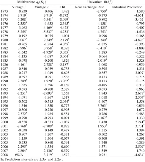
The prediction of instability is remarkable. The test picks up all the recessions, the oil price shocks, the stock market crash, the Asian crisis and the recent financial crisis.
Except for the 1991 and 2001 recessions, qi(Dk)> 3. The size of the sudden
jumps has clearly been relatively smaller (i.e., between 2) in the 1980s and 1990s
compared with the 1970s seem consistent with the Great Moderation story. See Bernanke (2004) on a discussion and full references of the research in this area.
For completeness, a univariate statistic for sudden and large jumps in the conditional variances could be used in addition to the multivariate statistic to test each of the three time series, individually. This will shed closer light on instability.
We compute the followings in order:
2 2
/ ) 1
( i i
i n S
V ; (12)
) (
1 i i n
i H V
u ; and (13)
) ( )
( 2 1
i i
i S u
R (14)
WhereVi is the statistic for a sudden shift in the variance, which is distributed
chi-squared, 2
i
S is the sample variance, niis the number of observation or the window for
which the variance is computed; 2is a pooled or overall variance calculated as
m i i ii S n m
n 1 2 / ) 1
( , where iis the number of samples =1,2,m. We map Vi onto a
standard normal distribution to make the presentation of the results easy. H(.)is the
distribution function of the chi-squared random variable with ni 1
The statistics are reported in table 1, columns 4-6 and plotted in figures 4, 5 and 6. They are the prediction intervals for the instability in the price of oil, the real exchange rate and the industrial production index individually.
In figure 4, the conditional variance for the real price of oil jumps high showing significant instability during the first and second oil price shocks as expected. A very large spike is recorded in 1986 and the stock market crashed in October 1987 then it signalled a sudden large shift in 1990 the year Iraq invaded Kuwait and the collapse of
the USSR. It signalled a shift 2 in 1992 and again in 1995. The statistic did not signal the recessions except 1991 and the recent one related to the financial crisis. From 1996 onward the statistic predicted no significant instability in the price of oil.
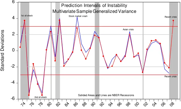
Figure 5 plots the prediction intervals for the real exchange rate depreciation. Relatively fewer sudden and large jumps in the conditional variance are recorded.
Again, the period up to 1982 shows significant activities at 2 and 3, which include the oil price shocks and the switching from the Bretton-Woods to free
floating. In 1985 it reacted again, but only by 2. This period is during the Reagan
administration when the US appreciated significantly; followed by another small signal in 1993 and by a large jump in 1996. These were followed by more less significant sudden shifts in 1999 – 2001 recession.
Both the price of oil and the real exchange rate exhibited more or less similar instability. The real exchange rate instability continued to the mid and late 1990s while oil's instability ceased in mid 1990s as if it is no longer an interesting variable. More intriguing is that neither the price of oil nor the real exchange rate signalled the recent financial crisis. This result does not seem to be consistent with Melvin and Taylor's (2009) who identified a foreign exchange crisis. Note that Melvin and Taylor (1) do not examine the real exchange rate but rather an index; (2) they do not provide a test statistic for conditional volatility. Thus they could have reported changes, but they did not test for their significance.
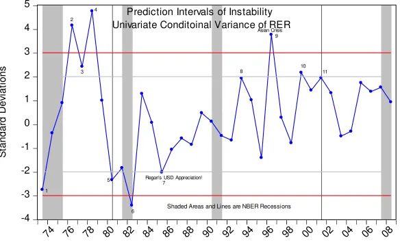
Figure 6 plots the univariate ( 2) i
S
R statistic for the industrial production. It signalled
crisis signalling in 2007 and more significantly so in 2008. Like the other two
variables it reacted to the first and the second oil price shocks with significant sudden and large increase. Then nothing significant happened until 2001 and 2006-2008. In between, the real economy seemed only agitated, with less significant sudden
increases in the conditional variance in 1993-1994.
A few interesting observations emerge from all these tests (univariate and
multivariate), which underscore the importance of using all of them for completeness. First, in 1984 and 1985 during the Reagan administration the US dollar appreciated to
its highest level, the multivariate qi(Dk)test statistic showed no significant change in
the conditional variance of the system. However, both the price of oil and the real exchange rate signalled significant instability in 1984 and in 1985 respectively.
Second, the multivariate statistic qi(Dk)signalled the Asian crisis in 1998 with a
jump > 2, but non of the three univariate statistics were significant in 1998. This
finding might be consistent with Fernandez (2006). Fernandez (2006) like Malik (2003) uses an iterated Cumulated Sums of Squares (ICSS) logarithm and fined no significant permanent change in volatility after the Asian crisis and 9/11. The real exchange rate only signalled a large jump in 1996, but one cannot be sure whether this was related to the Asian crisis because nothing happened until it jumped again at the
2
level in 1999. Third, most intriguing is that the tests signalled a jump in 2001 with different levels of significance, except the price of oil, and none of the tests picked up the US invasion of Iraq in 2003 obviously because it was an anticipated shock. Fourth, while the multivariate test statistic picked up signs of the current crisis from 2006 and showed significant jumps in the conditional variance of the system in 2006-2008, the univariate test statistic for the industrial production reacted
significantly, but no signals came from the univariate test statistics for oil prices and the real exchange rate.
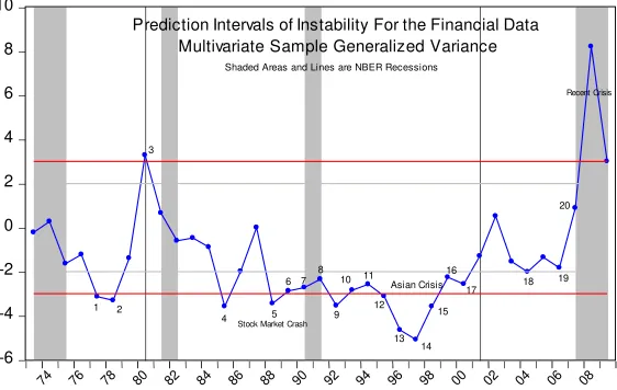
Figure 7 plots the qi(D)Multivariate Sample Generalized Variance for four financial
series are from January 1973 to December 2009. We keepn30,
thusk1m37.
Interestingly, the test showed no significant change during the first oil shock period while all other variables reacted significantly. However, it picked up the 1980; 1990 and the most recent recession. The signal of the recent financial crisis is particularly large. It signalled the stock market crash and the Asian crisis.
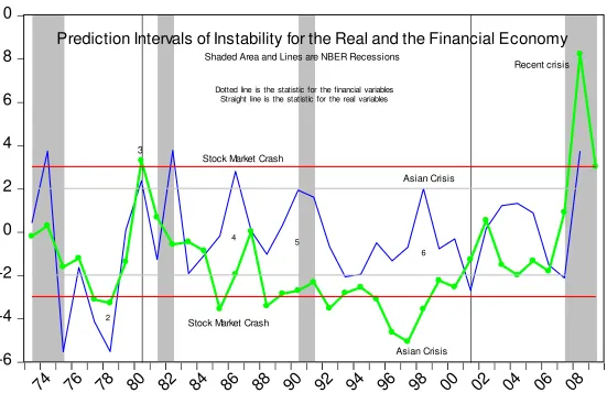
Figure 8, combines the test statistics for the real economic and the nominal financial data. There is a general agreement among the two. They signalled, albeit with different degrees of significance, the second oil shock. The real variables reacted stronger. Both the real and the nominal variables reacted to the 1980's recession; to the stock market crash; the Asian and the recent financial crisis.
In addition to these monthly frequency sudden large shifts in the conditional variance (either multivariate or univariate), the central bank staff can analyze daily data. Most of the useful daily data are financial market data. Then they match the daily
predictions and the monthly predictions, see Razzak (1991).
4. Conclusion
We introduce a multivariate test statistic to test for sudden and large shits in the conditional variance of some stationary Gaussian random variables, which when used to test particular data could give an early alarm about systemic risk. The multivariate statistic is based on the Sample Generalized Variance, Anderson (1958) extended to handle-variates.
We used US monthly real data from two vintages from 1973 to 2008. We argued that central banks could use this machinery to predict and study instability. They might be able to be ready for crisis since the probabilistic prediction intervals provided by the statistics are very accurate.
and 1973 to 2008 (the second vintage of the data) show that the 1970s and 1980s are statistically significantly less stable than the rest of the sample, which is consistent with the Great Moderation story, e.g., Bernanke (2004). The statistics accurately predicted the first and the second oil shocks. They also predicted the US recessions. They sent alarms before the stock market crash, the Asian crisis and the most recent financial crisis. The multivariate statistic began, unlike the univariate test statistics, to sound a series of alarm signals regarding the recent crisis. The first signal went off in 2006, 2007 and finally a very large signal in 2008.
These tests are easy to use. They could be used to test a single time series, a bi-variate system of two time series, and a multibi-variate system of more than 2 and up to
References
Anderson, T. W., Introduction to Multivariate Statistical Analysis, New York, John Wiley (1958).
Bernanke, B., "The Great Moderation," Speech at the Meeting of the Eastern Economic Association, (2004), Washington, DC.
Chen, J. and A. K. Gupta, “Testing and Locating Variance Changpoint with
Application to Stock Prices,” Journal of The American Statistical Association, 92, No. 438, (1997), 739-747.
Fernandez, V., "The Impact of major Global Events on Volatility Shifts: Evidence from The Asian Crisis and 9/11," Economic Systems, 30, (2006), 79-97.
Ganadesikan, M. and S. S. Gupta, "A Selection Procedure for Multivariate Normal Distribution in Terms of the Generalized Variance," Technometrics, 12, (1970), 103-116.
Inclan, C. and G. C. Tiao, “Use of Cumulative Sums of Squares for Retrospective Detection of Changes of Variance,” Journal of The American Statistical Association 89, No. 427, (1994), 913-923.
Kamisky, C., S. Lizondon, and C. Reinhart, "Leading Indicators of Currency Crisis," Staff Paper 1, IMF, (1998).
Malik, F., "Sudden Changes in variance and Volatility Persistence in Foreign
Exchange Markets," Journal of International Financial Management, 13, (2003), 217-230.
Melvin, M. and M. Taylor, "The Crisis in the Foreign Exchange Market," CESIFO Working Paper No. 2707, (2009).
Razzak, W. A., "Target Zone Exchange Rate," Economics Letters 35, (1991), 63-70.
Reinhart, C. and K. Rogoff, "Is the 2007 U.S. Sub Prime Financial Crisis So
Different? An International Historical Comparison, Working Paper, School of Public Policy at the University of Maryland, (2008).
Shewhart, W.G., Economic Control of Quality Manufactured Products, New York, De van Nostrand Co., Inc. (1931).
Taleb, N. N., The Black Swan: The Impact of the Highly Improbable, New York, Random House, (2007).
Taylor, J. and J. C. Williams, "A Black Swan in the Money Market," American Economic Journal Macroeconomics, Volume 1, No.1, (2009), 58-83.
Table 1: Multivariate Sample Generalized Variance and Univariate Test Statistic for Sudden and large shifts in the conditional variance
Multivariate qi(Dk) Univariate ( )
2
i
S R
Vintage 1 Vintage 2 Oil Real Exchange Rate Industrial Production
1973 0.939 0.406 1.482 -2.750# 1.580
1974 3.719* 3.719* -8.272* -0.373 -4.651*
1975 -5.208* -5.541* 8.099* 0.892 -3.462*
1976 -2.353# -1.653 2.345# 4.158* 0.795
1977 -3.962 -4.169* 4.423* 2.425# 0.407
1978 -5.255* -5.537* 4.753* 4.753* -1.536
1979 0.192 0.075 1.001 0.996 0.365
1980 3.067* 2.349# 2.179# -2.340# -4.826*
1981 -0.765 -1.284 4.055* -1.835 -0.393
1982 3.996* 3.758* 0.393 -3.410* -1.808
1983 -1.642 -1.929# 3.055* 1.283 -0.249
1984 -1.135 -1.087 3.064* 0.064 0.522
1985 -0.078 -0.200 1.829 -2.019# 1.328
1986 4.161* 2.788# -5.187* -1.068 0.959
1987 0.840 0.039 0.755 -0.595 1.231
1988 -0.217 -1.049 0.693 -0.857 3.097*
1989 0.397 0.291 1.538 0.473 0.715
1990 2.389# 1.920# -3.962* 0.113 0.175
1991 1.635 1.596 -0.162 -0.485 0.312
1992 -0.673 -0.700 2.329 -0.673 0.963
1993 -2.251# -2.093# 1.563 1.943 2.673#
1994 -1.071 -1.967 1.317 1.018 2.503#
1995 -0.502 -0.515 2.044# -1.407 1.558
1996 -1.346 -1.350 0.777 3.763* 0.056
1997 -0.506 -0.720 0.995 0.279 1.672
1998 2.372# 1.985 0.554 -0.786 -0.583
1999 -0.790 -0.793 0.091 2.167# 1.330
2000 -0.528 -0.333 -1.037 1.430 2.241#
2001 -2.768# -2.709# 0.972 1.953# 3.731*
2002 -0.038 0.149 0.477 1.315 1.394
2003 0.907 1.207 -0.371 -0.502 1.267
2004 1.159 1.304 -0.057 -0.300 0.591
2005 0.733 0.860 0.591 1.740 -0.889
2006 -2.295# -1.534 0.690 1.371 2.509#
2007 -2.804# -2.136# 0.579 1.549 1.740
2008 #N/A 3.719* 1.572 0.931 -4.634*
The Prediction intervals are 3 and 2.
* Values of the tests > 3 denote significant sudden and large shifts in the conditional variance.
Figure 1: West Texas Oil Price dollar per barrel October 1972-September 2009
0.00
20.00
40.00
60.00
80.00
100.00
120.00
140.00
160.00
WTO price
Figure 2: Re al We st Te xas Oil Price Change s and U.S. Re ce ssions
1973 1976 1979 1982 1985 1988 1991 1994 1997 2000 2003 2006 -40
[image:21.842.119.773.171.400.2]Figure 3
Solid Line is Data 2007 Vintage and Dotted Line is Data 2008 Vintage
-6
-4
-2
0
2
4
6
74
76
78
80
82
84
86
88
90
92
94
96
98
00
02
04
06
08
Prediction Intervals of Instability
Multivariate Sample Generalized Variance
Sahded Areas and Lines are NBER Recessions
1st oil shock
2nd oil shock
Stock market crash
Asian crisis
Recent crisis
Recent crisis
S
ta
n
d
a
rd
D
e
vi
a
ti
o
n
Figure 4
-7.5
-5.0
-2.5
0.0
2.5
5.0
7.5
74
76
78
80
82
84
86
88
90
92
94
96
98
00
02
04
06
08
S
ta
n
d
a
rd
D
e
vi
a
ti
o
n
[image:23.842.97.743.113.485.2]s
Prediction Intervals of Instability
Univariate Conditional Variance for Oil Price
Shaded Ares and Lines are NBER Recessions
Stock Market Crash
1 2
3
4 5
6 7
10 8 9
Oil shock
2nd Oil shock
11
12 13
Figure 5
-4
-3
-2
-1
0
1
2
3
4
5
74
76
78
80
82
84
86
88
90
92
94
96
98
00
02
04
06
08
S
ta
n
d
a
rd
De
vi
a
ti
o
n
s
Prediction Intervals of Instability
Univariate Conditoinal Variance of RER
Shaded Areas and Lines are NBER Recessions
Asian Crisis
Regan's USD Appreciation!
1
2
3 4
5
6
7
8
9
Figure 6
-5
-4
-3
-2
-1
0
1
2
3
4
74
76
78
80
82
84
86
88
90
92
94
96
98
00
02
04
06
08
Prediction Intervals of Instability
Univariate Conditional Variance for Industrial Production
Shaded Areas and Lines are NBER Recessions
S
ta
n
d
a
rd
De
vi
a
ti
o
n
s
Stock Market Crash
1 2
3
4 5
6
7 8
9
Figure 7
-6
-4
-2
0
2
4
6
8
10
74 76 78 80 82 84 86 88 90 92 94 96 98 00 02 04 06 08
Prediction Intervals of Instability For the Financial Data
Multivariate Sample Generalized Variance
Shaded Areas and Lines are NBER Recessions
1 2 3
4 5
6 7 8
9 10 11
12
13 14
15 16
17 18
19 Asian Crisis
Stock Market Crash
Recent Crisis
Figure 8
-6
-4
-2
0
2
4
6
8
10
74
76
78
80
82
84
86
88
90
92
94
96
98
00
02
04
06
08
Prediction Intervals of Instability for the Real and the Financial Economy
3
Recent crisis
2
4
Stock Market Crash
Asian Crisis
5
6
Stock Market Crash
Asian Crisis Shaded Area and Lines are NBER Recessions
SAS-IML Code to compute qi(Dk)
%macro razzak(dataset=stability, Variables=X1 X2 X3, m=36, n=12); proc iml;
use &dataset;
read all into x var {&variables};
m=&m;/*-number of samples-*/
n=&n; /*- sample sizer-*/
p=ncol(x); /*-number of variables-*/
t=nrow(x); /*-total number of observation-*/
b=j(n,1,1);
j=(p-1)*(p-2)/(2*n);
scale=(p/2)*(1-j)##(1/p);
shape= p*(s-p)/2 ;
start qc;
do h=n to t by n;
gp=x(|(h-n+1):h,|);
if h=n then xb=mgp; else xb=xb//mgp;
cssg=gp-(mgp@b);
ssg=(cssg`*cssg);
covg=(cssg`*cssg)/((n)-1);
dcovg=det(covg);
if h=n then do ;
ssp=ssg;;dcov=dcovg ; end;
else do ;ssp=ssp+ssg;dcov=dcov//dcovg; end;
end;
xdb=x(|:,|)@b;
b=j(m,1,1);
cov=ssp/(t-m);/* this is a S bar matrix)*/
dsbar=det(cov);
gamma=((n-1)*p)*(dcov/dsbar)##(1/p);
y=gamma/scale;
gamma=probgam(y,shape);
t2=(n*diag((xb-xdb)*inv(cov)*(xb-xdb)`))(|,+|);
sample=(1:m);
colchr={'Z1' 'Z2' 'Z3' 'Z4' 'Z5' 'Z6' 'Z7' 'Z8' };
u=probchi(t2,p);
q=probit(u);
u1=probgam(y,shape);
q1=probit(u1); /* This is q(D) statistic, which is distributed standard normal*/
output2=output2//(sample`||gamma||u1||q1);
colchr2={'Sample' 'Gam' 'u1' 'Q1'};
output=output//(sample`||t2||u||q||dcov);
colchr1={'SAMPLE' 'T SQUARE' 'U' 'Q' 'DET n'};
*print cov(|colname=colchr rowname=colchr|);
* print output(|colname=colchr1|);
* print output2(|colname=colchr2|) ;
create p0 from output(|colname=colchr1|);
append from output;
create p1 from output2(|colname=colchr2|);
append from output2;
close p1; finish ; start main; run qc; finish; run main ; quit;
proc print data=p0;
title2'IML OUTPUT Dataset=P0'; run;
proc print data=p1;
title2'IML OUTPUT Dataset=P1'; run;
%mend;
An R code in case one does not have SAS. This software is free.
This is the RUN file.
Create a folder Prog in the C drive.
Save the R code written below in boldface in the Prog folder and name it Prog.R Create a file data.txt and save in the Prog folder in the C drive
Download R from the net and save in the Prog folder in the C drive.
RUN.txt
setwd("c:/prog") source("prog.R")
stability <- read.table("data.txt", header=TRUE)
out <- test(dataset=Name , variables=c("X1", "X2", "X3"), m=Number,n=Number) out$p0
out$p1
Code: Prog.R
test <- function(dataset, variables, m, n) {
x <- dataset[,charmatch(variables, colnames(dataset))] p <- ncol(x)
t <- nrow(x) b <- matrix(1, n, 1) j <- (p-1)*(p-2)/(2*n) scale <- (p/2)*(1-j)^(1/p) shape <- p*(n-p)/2
xb <- mgp } else {
xb <- rbind(xb,mgp) }
cssg <- as.matrix(gp-(mgp %x% b)) ssg <- (t(cssg) %*% cssg)
covg <- (t(cssg) %*% cssg)/((n)-1) dcovg <- det(covg)
if (h==n) { ssp <- ssg dcov <- dcovg
} else {
ssp <- ssp+ssg
dcov <- rbind(dcov, dcovg) }
}
#xdb=colMeans(x)
cov <- ssp/(t-m) #/* this is a S bar matrix*/
dsbar <- det(cov);
gamma <- as.vector(((n-1)*p)*(dcov/dsbar)^(1/p)) y <- gamma/scale
gamma <- pgamma(y,shape=shape) b <- matrix(1, m, 1)
xdb <- t(colMeans(x)) %x% b
t2 <- n*diag((xb-xdb)%*%solve(cov)%*%t(xb-xdb)) sample <- 1:m
colchr <- c('Z1', 'Z2', 'Z3', 'Z4', 'Z5', 'Z6', 'Z7', 'Z8') u <- pchisq(t2,p)
q <- qnorm(u)
u1 <- pmin(pgamma (y,shape), 0.999999) /*We do this to avoid having U1=1*/
q1 <- qnorm(u1)
colchr2 <- c('Gam', 'u1', 'Q1')
output <- data.frame(t2=t2,u=u,q=q,dcov=as.vector(dcov)) colchr1 <- c( 'T SQUARE', 'U', 'Q', 'DET N')
colnames(output) <- colchr1 colnames(output2) <- colchr2
return(list(p0=output, p1=output2, xdb = xdb)) }
i Think of a
3
which constitute a probability of 0.9973, hence 1-0.9973.
ii In some particular data one can think of this as a measure of systemic risk.
iiiAnderson (1958) shows that the determinant of S2 is proportional to the sum of squares of
the volumes of all parallelotopes formed by using as principle edgesvectors of X1,X2,X
as one set of end points, and the mean ofXas the other with
1) (
1
n as the factor of
proportionality.
iv For a two-variable case, i.e., 2, the appropriate prediction intervals are derived such that the statistic is an approximately chi-squared random variable, when the number of degrees of freedom for estimating the parameters is large. When the number of degrees of freedom is nor large, the statistic is an approximately HotellingT2. This is easily computed given the definitions above:
( ) ( ) 2 ( )( )
1 2 2 1 1 2 2 2 2 1 1 2 2 s x x s x x s x x s x x n T
, whereis the correlation coefficient
and x,x,s as defined earlier.
v
Chebyshev's inequality (also known as Tchebysheff's inequality, Chebyshev's theorem, or the Bienaymé-Chebyshev inequality) states that in any data sample or probability distribution, nearly all the values are close to the mean value, and provides a quantitative description of nearly all and close to, For anyk1, the following example (where 1/k) meets the bounds exactly. So Pr(X 1)1/2k2; Pr(x0)11/k2and Pr(X 1)1/2k2for that
distributionPr(|X|)k 1/k2. Equality holds exactly for any distribution that is a linear transformation of this one. Inequality holds for any distribution that is not a linear