E
s s a y s
o n
E
s t i m a t i o n
a n d
I
n f e r e n c e
f o r
V
o l a t i l i t y
w i t h
H
i g h
F
r e q u e n c y
D
a t a
Il z e Ka l n i n a
A Di s s e r t a t i o n
Pr e s e n t e d t o t h e De p a r t m e n t o f Ec o n o m i c s o f Lo n d o n Sc h o o l o f Ec o n o m i c s a n d Po l i t i c a l Sc i e n c e
in Ca n d i d a c y f o r t h e De g r e e o f Do c t o r o f Ph i l o s o p h y
UMI Number: U615957
All rights reserved
INFORMATION TO ALL USERS
The quality of this reproduction is dependent upon the quality of the copy submitted.
In the unlikely event that the author did not send a complete manuscript
and there are missing pages, th ese will be noted. Also, if material had to be removed, a note will indicate the deletion.
Dissertation Publishing
UMI U615957
Published by ProQuest LLC 2014. Copyright in the Dissertation held by the Author. Microform Edition © ProQuest LLC.
All rights reserved. This work is protected against unauthorized copying under Title 17, United States Code.
ProQuest LLC
789 East Eisenhower Parkway P.O. Box 1346
D eclaration
I certify th at the thesis I have presented for examination for the M Phil/PhD
degree of the London School of Economics and Political Science is solely my own
work other than where I have clearly indicated th a t it is the work of others (in which
case the extent of any work carried out jointly by me and any other person is clearly
identified in it).
The copyright of this thesis rests with the author. Quotation from it is perm itted,
provided th at full acknowledgement is made. This thesis may not be reproduced without the prior w ritten consent of the author.
I warrant th at this authorization does not, to the best of my belief, infringe the rights of any third party.
© Copyright by Ilze Kalnina, 2009.
A bstract
Volatility is a measure of risk, and as such it is crucial for finance. But volatility is
not observable, which is why estimation and inference for it are im portant. Large
high frequency data sets have the potential to increase the precision of volatility esti
mates. However, this d ata is also known to be contam inated by market microstructure
frictions, such as bid-ask spread, which pose a challenge to estimation of volatility.
The first chapter, joint with Oliver Linton, proposes an econometric model th at
captures the effects of market m icrostructure on a latent price process. In particular,
this model allows for correlation between the measurement error and the return pro
cess and allows the measurement error process to have diurnal heteroskedasticity. A
modification of the TSRV estim ator of quadratic variation is proposed and asymptotic distribution derived.
Financial econometrics continues to make progress in developing more robust and
efficient estimators of volatility. But for some estimators, the asymptotic variance is hard to derive or may take a complicated form and be difficult to estimate. To
tackle these problems, the second chapter develops an autom ated m ethod of inference th at does not rely on the exact form of the asymptotic variance. The need for a
new approach is motivated by the failure of traditional bootstrap and subsampling
variance estimators with high frequency data, which is explained in the paper. The
main contribution is to propose a novel way of conducting inference for an im portant
general class of estimators th at includes many estim ators of integrated volatility. A
subsampling scheme is introduced th a t consistently estimates the asymptotic variance
for an estimator, thereby facilitating inference and the construction of valid confidence
intervals.
The third chapter shows how the multivariate version of the subsampling method
A cknow ledgem ents
I am deeply indebted to my supervisor Oliver B. Linton for his help, encouragement,
and guidance throughout my PhD studies. I am grateful to Peter C. B. Phillips
for hosting me at the Cowles Foundation and all the support and inspiration I have
received there.
C ontents
D e c la r a tio n ... ii
A b s tr a c t... iii
A cknow ledgem ents... iv
1 E stim ation o f Q u ad ratic V ariation in th e P r esen ce o f D iurnal and H etero sced a stic M easu rem en t Error 1 1.1 In tro d u c tio n ... 1
1.2 The M o d e l... 5
1.3 E stim a tio n ... 10
1.4 Asymptotic P r o p e r t i e s ... 13
1.5 Simulation s t u d y ... 18
1.6 Empirical an aly sis... 23
1.6.1 The D a t a ... 23
1.6.2 Estim ation of a ... 24
1.6.3 Estim ation of Scedastic function c u ( . )... 25
1.6.4 Estim ation of Quadratic V ariation... 26
1.7 Conclusions and E x te n s io n s ... 28
2 Subsam pling H ig h Frequency D a ta 30 2.1 In tro d u c tio n ... 30
2.2.1 Failure of the Traditional Resampling S chem es... 38
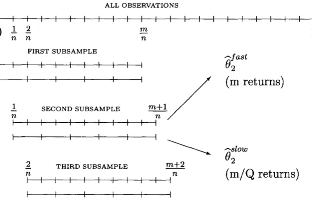
2.2.2 The New Subsampling Schem e... 40
2.2.3 An Alternative Subsampling S c h e m e ... 43
2.3 Inference for the Two Scale Realized Volatility E s tim a to r ... 46
2.4 Inference for a General E s tim a to r ... 55
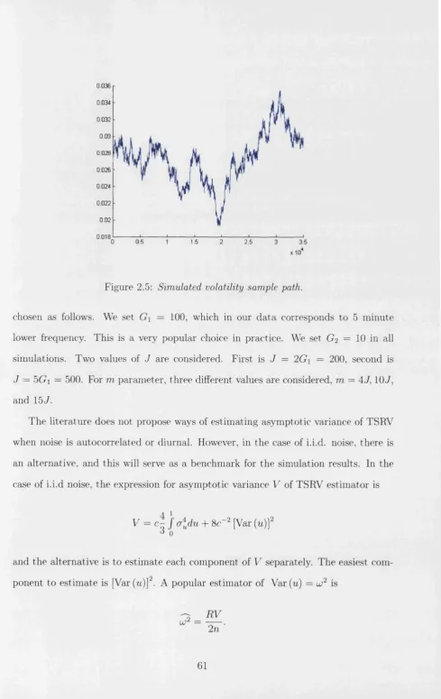
2.5 Simulation S t u d y ... 59
2.6 Empirical A n a l y s is ... 64
2.7 Conclusion ... 66
3 S u b sam p ling and T im e V ariation in B e ta s 67 3.1 In tro d u c tio n ... 67
3.2 Realized B e t a ... 68
3.2.1 Estim ation of beta: noise-free and synchronous d a t a ... 69
3.2.2 Estim ation of beta: noisy and asynchronously observed d ata . 71 3.2.3 Testing for constant b e t a s ... 74
3.3 M ultivariate S u b s a m p lin g ... 76
3.4 Empirical A n a l y s is ... 78
3.4.1 The D a t a ... 79
3.4.2 R e su lts... 80
3.5 Simulation S t u d y ... 83
3.6 Conclusion ... 85
A A p p en d ices for C h ap ter 1 95 A .l Proof of Theorem 1 .4 .1 ... 95
A.2 Technical Appendix to Chapter 1 ... 100
A.2.1 L e m m a s ... 104
A.2.2 Proofs of L em m as... 106
B A p p en d ices for C h ap ter 2 128
B .l Proofs of Chapter 2 ... 128
B.1.1 Proof of Proposition 1 ... 129
B.1.2 Proof of Proposition 2 ... 130
B .l.3 Proof of Proposition 3 ... 135
B.1.4 Proof of Theorem 2 .3 .1 ... 141
B.1.5 Proof of Lemma 2 .3 .2 ... 146
B.1.6 Proof of Theorem 2 .4 .1 ... 147
B.2 Tables and Figures of Chapter 2 ... 149
C hapter 1
E stim a tio n o f Q uadratic V ariation
in th e P resen ce o f D iurnal and
H etero sced a stic M easurem ent
Error
1.1
Introduction
It has been widely recognized th at using very high frequency data requires taking
into account the effect of market m icrostructure (MS) noise. We are interested in the estimation of the quadratic variation of a latent price in the case where the observed
log-price Y is a sum of the latent log-price X th a t evolves in continuous time and an
error u th a t captures the effect of MS noise.
There is by now a large literature th a t uses realized variance as a nonparametric
measure of volatility. The justification is th a t in the absence of market microstructure
noise it is a consistent estim ator of the quadratic variation as the time between ob
(2007). In practice, ignoring microstructure noise seems to work well for frequencies
below 10 minutes. For higher frequencies realized variance is not robust, as has been
evidenced in the so-called ‘volatility signature plots’, see, e.g. Andersen et al. (2000). The additive measurement error model where u is independent of X and i.i.d.
over time was first introduced by Zhou (1996). The usual realized volatility estim a
tor is inconsistent under this assumption. The first consistent estim ator of quadratic
variation of the latent price in the presence of MS noise was proposed by Zhang,
Mykland, and Ai't-Sahalia (2005a) who introduced the Two Scales Realized Volatility
(TSRV) estimator, and derived the appropriate central limit theory. TSRV estimates the quadratic variation using a combination of realized variances com puted on two
different time scales, performing an additive bias correction. It has a rate of conver
gence n -1/6. Zhang (2004) introduced the more complicated Multiple Scales Realized
Volatility (MSRV) estimator th at combines multiple (~ n 1/2) time scales, which has a convergence rate of n -1/4. This is known to be the optimal rate for this problem.
Both papers assumed th at the MS noise was i.i.d. and independent of the latent price. This assumption, according to an empirical analysis of Hansen and Lunde
(2006), ’’seems to be reasonable when intraday returns are sampled every 15 ticks or
so” . Further studies have tried to relax this assumption to allow modelling of even
higher frequency returns. Ai't-Sahalia, Mykland and Zhang (2006a) modify TSRV and MSRV estimators and achieve consistency in the presence of serially correlated MS
noise. Another class of consistent estimators of the quadratic variation was proposed
by Barndorff-Nielsen, Hansen, Lunde, and Shephard (2006). They introduce realized
kernels, a general class of estimators th at extends the unbiased but inconsistent esti
mator of Zhou (1996), and is based on a general weighting of realized autocovariances
as well as realized variances. They show th at realized kernels can be designed to be
consistent and derive the central limit theory. They show th a t for particular choices
mators, or even more efficient. Apart from the benchmark setup where the noise is
i.i.d. and independent from the latent price Barndorff-Nielsen et al. (2006) have two
additional sections, one allowing for AR(1) structure in the noise, another with an
additional endogenous term albeit one th at is asymptotically degenerate.
We generalize the standard additive noise model (where the noise is i.i.d. and independent from the latent price) in three directions. The first generalization is
allowing for (asymptotically non-degenerate) correlation between MS noise and the
latent returns. This is motivated by a paper of Hansen and Lunde (2006), where,
for very high frequencies: ’’the key result is the overwhelming evidence against the
independent noise assumption. This finding is quite robust to the choice of sampling
method (calendar-time or tick-time) and the type of price d ata (transaction prices or quotation prices)” .1
Another generalization concerns the magnitude of the MS noise. All of the papers
above, like most of related literature, assume th at the variance of the MS noise is constant and does not change depending on the tim e interval between trades. We
call this a large noise assumption. We explicitly model the magnitude of the MS noise
via a param eter a , where the a = 0 case corresponds to the benchmark case of large noise. We allow also a > 0 in which case the noise is ’’small” and specifically the
variance of the noise shrinks to zero with the sample size n. The rate of convergence
of our estim ator depends on the magnitude of the noise, and can be from n-1 /6 to
n -1/3, where n-1/6 is the rate of convergence corresponding to the ’’big” noise case
when a = 0.
How could the size of the noise ’’depend” on the sample size? We give a fuller
discussion of this issue below, but we note here two arguments. First, there is a
negative relationship between the bid-ask spread (an im portant component of the
MS noise for transaction data) and a number of (other) liquidity measures, including
number of transactions during the day. This negative relationship is a stylized fact
from the market m icrostructure literature. See, for example, Copeland and Galai
(1983) and Mclnish and Wood (1992). Also, Awartani, Corradi and Distaso (2004)
write th at ” an alternative model of economic interest [to the standard additive noise
model] would be one in which the microstructure noise variance is positively correlated
with the time interval” . This is in principle a testable hypothesis. Using Dow Jones
Industrial Average data, the authors test for and reject the hypothesis of constant
variance of the MS noise across frequencies.
The third feature of our model is th at we allow the MS noise to exhibit diurnal heteroscedasticity. This is motivated by the stylized fact in market microstructure
literature th a t intradaily spreads and intradaily stock price volatility are described typically by a U-shape (or reverse J-shape). See Andersen and Bollerslev (1997),
Gerety and Mulherin (1994), Harris (1986), Kleidon and Werner (1996), Lockwood
and Linn (1990), and Mclnish and Wood (1992). Allowing for diurnal heteroscedastic ity in our model has the effect th a t the original TSRV estim ator may not be consistent
because of end effects. In some cases, instead of estim ating the quadratic variation,
it would be estimating some function of the noise. We propose a modification of the
TSRV estimator th at is consistent, without introducing new param eters to be chosen.
Our model is not meant to be definitive and can be generalized in a number of ways.
The structure of the paper is as follows. Section 2 introduces the model. Sec
tion 3 describes the estimator. Section 4 gives the main result and the intuition
behind it. Section 5 investigates the numerical properties of the estim ator in a set
of simulation experiments. Section 6 illustrates the ideas with an empirical study of
IBM transaction prices. Section 7 concludes. We use ==>- to denote convergence in
1.2
The M odel
Suppose th at the latent (log) price process { X u t G [0, T]} is a Brownian semimartin-
gale solving the stochastic differential equation
d X t = fLtdt + a tdWu ( i.i)
where W t is standard Brownian motion, /it is a locally bounded predictable drift
function, and a t a cadlag volatility function; both are independent of the process
{W tl t G [0, T]}. The (no leverage) assumption of {at , t G [0, T } being independent
of {W t, t G [0, T]}, though reasonable for exchange rate data, is unrealistic for stock price data. However, it is frequently used and makes the theoretical analysis more tractable. The simulation results suggest th at this assumption does not change the
result. Furthermore, in many other contexts the presence of leverage does not affect the limiting distributions, see Barndorff-Nielsen and Shephard (2002).
The additive noise model says th a t the noisy price Y is observed at times i i , . . . , tn
on some fixed domain [0, T]
where uti is a random variable representing measurement error. W ithout loss of much
generality we are going to restrict attention to the case of equidistant observations
with T —1. This type of model was first introduced by Zhou (1996) who assumed
th at uti is i.i.d. over i and independent of { X t , t G [0,1]}. In this case the signal to
noise ratio for returns decreases with sample size, i.e., var(A X tJ /v a r ( Auti) —>0 as
n —> oo, and at a specific rate such th at lim ^o o nvar(A X tJ /v a r(A u tJ < oo, which
implies inconsistency of realized volatility. We are going to modify the properties of
the process { r ^ } and its relation to { X u t G [0,1]}.
We would like to capture the idea th a t the measurement error can be small. This
can be addressed by adopting a model u ti = where eti is an i.i.d. sequence with mean zero and variance one, and a £ is a param eter such th at a € —► 0. Many
authors have found small <re in practice. As usual one wants to make inferences
about data drawn from the true probability measure of the d ata where both n is
finite and a e > 0 by working with a limiting case th at is more tractable. In this
case there are a variety of limits th at one could take. Bandi and Russell (2006a) for
example calculate the exact MSE of the statistic of interest, and then in equation
(24) implicitly take <7e —> 0 followed by n —► oo. We instead take the sound and
well established practice in econometrics of taking pathwise limits, th a t is we let
a € = o e(n) and then let n —> oo. Such a limit w ith ”small” noise has been used before to derive Edgeworth approximations (Zhang et al., 2005b), to calculate optimal
sampling frequency of inconsistent estim ator for QVX (Zhang et al., 2005a, eqn. 53),
to estimate QVX consistently when X follows a pure jum p process and Y is observed fully and continuously (Large, 2007), and to estim ate QVX consistently in a pure
rounding model (Li and Mykland, 2006; Rosenbaum, 2007). An example from MS modelling literature in microeconomics is Back and Baruch (2004) who show the
link between the two key papers in asymmetric information modelling, Glosten and
Milgrom (1985) and Kyle (1985) using a limit with small noise. In particular, they
consider a limit of Glosten and Milgrom (1985) as the arrival rate of trades explodes
(so the number of trades in any interval goes to infinity) and order size (and hence incremental information per trade) goes to zero, thus reaching the Kyle (1985) model
as a limit. We are also mindful not to preclude the case where <re(n) is ’’large” i.e.,
We next present our model. We assume th at
U ti = vt i + E ti (1.3)
vtl = s
1
„(Wi,-Wii_1)
eti = m (ti) + n~a/2w (U) eti, a G [0 ,1 /2 )
with eti i.i.d. mean zero and variance one and independent of the Gaussian process
{W u t e [0,1]} with E\eti\4+v < oo for some 77 > 0. The functions m and u are
differentiable, nonstochastic functions of time. They are unknown as are the constants
S and a. The usual benchmark measurement error model with noise being i.i.d. and
independent from the latent price has a = 0, 7n = 0 and u(.) and ra(.) constant (see, e.g., Barndorff-Nielsen and Shephard (2002), Zhang et al. (2005a) and Bandi and
Russell (2006b)).
The process for the latent log-price is motivated by the fundamental theory of asset prices, which states th at, in a frictionless market, log-prices must obey a semi
martingale; we are specializing to the Brownian semimartingale case (1.1). We want
to model log-prices at very high frequency where frictions are im portant and observed prices do not follow a semimartingale. One way of partly reconciling the evidence in
volatility signature plots of the price behavior in very high and moderate frequencies
is to assume th a t observed prices can be decomposed as in (1.2). The first component
X is a semi-martingale with finite quadratic variation, while the second component
u is not a semi-martingale and has infinite quadratic variation. In particular, the
increments in u are of larger magnitude than th a t of X , and this difference is the
key in identifying the quadratic variation of X . We split the noise component u into
an independent term e th a t has been considered in the literature, and a 1-dependent
endogenous part v, which is correlated with X due to being driven by the same
martingale and having infinite quadratic variation, the main motivation of the way e is modelled.
There are three key parts to our model: the correlation between u and X, the
relative magnitudes of u and X , and the heterogeneity of u. We have E[uti] = m(ti)
and var[uti] = <5272 (£* — ^ _ i) + 2n~acr2(i/n). To have the variance of both terms in u
equal, we set 7 2 = n l~a. This seems like a reasonable restriction if both components
are generated by the same mechanism. In this case, both of the measurement error
terms are Op(n~a). In our model the signal to noise ratio of returns varies with sample
size in a way depending on a so th at only lim ^oo n1_Qvar(A X ti)/v ar(A u ti) < 00. We
exploit the fact th a t for consistency of the TSRV estim ator, it is enough to assume
th a t noise increments are of larger order of magnitude than the latent returns, and the usual stronger assumption limn_ 00 nvar(A X t .)/var(A uti) < 00 is not necessary.
The process eti is a special case of the more general class of locally stationary
processes of Dahlhaus (1997). The generalization to allowing time varying mean and variance in the measurement error allows one to capture diurnal variation in the
measurement error process, which is likely to exist in calendar time. Nevertheless, the measurement error in prices is approximately stationary under our conditions,
which seems reasonable.
The term v in u induces a correlation between latent returns and the change
in the measurement error, which can be of either sign depending on 5. Correlation
between u and X is plausible due to rounding effects, price stickiness, asymmetric
information, or other reasons [Bandi and Russell (2006c), Hansen and Lunde (2006),
Diebold (2006)].2 In the special case th at at = a and u (U) = u, we find
corr(AJVr(i, A u u ) ~ .
J[2<52 + 2u;2]
In this case, the range of correlation is limited, although it is quite wide - one can
obtain up to a correlation of ± l/ \ / 2 depending on the relative magnitudes of 8, u.
An alternative model for endogenous noise has been developed by Barndorff-
Nielsen, Hansen, Lunde, and Shephard (2006). In our notation, they have the en
dogenous noise part such th a t vai(vti) = 0 ( 1 /n) , and an i.i.d., independent from X
part w ith var(eti) = O (1). They conclude robustness of their estim ator to this type
of endogeneity, with no change to the first order asymptotic properties compared to
the case where vti = 0.
The focus of this paper is on estimating increments in quadratic variation of the
latent price process,3 but estimation of parameters of the MS noise in our model is also
of interest. We acknowledge th at not all the parameters of our model are identifiable.
In particular, the endogeneity parameter may not be identified unless one knows something about the distribution of e and in particular th a t it is not Gaussian.4
However, other parameters are identified. In Linton and Kalnina (2005) we provided
a consistent estimator of a , see also Section 6 here for empirical implementation and discussion. Estim ating the function uj (r) would allow us to measure the diurnal
variation of the MS noise. In the benchmark measurement error model this is a
constant u (r) = lj th a t can be estimated consistently by Y^=i O'Wi — Y u )2 / 2 n
(Bandi and Russell, 2006b; Barndorff-Nielsen et al., 2006; Zhang et al., 2005a). In
3There is a question about whether one should care about the latent price or the actual price. This has been raised elsewhere, see Zhang, Mykland, and Ait-Sahalia (2005). We stick with the usual practice here, acknowledging that the presence of correlation between the noise and efficient price makes this even more debatable, Ait-Sahalia, Mykland, and Zhang (2006b). Also, note that we are following the literature and estimating the quadratic variation of the latent log-price and not the latent price.
our model, instead of n ~ l, the appropriate scaling is n a~l . Such an estim ator would
converge to 82 + J oj2 (u ) du. Hence, this estimator would converge asymptotically to
the integrated variance of the MS noise. Following Kristensen (2006), in the special
case S = 0, we could also estimate u (•) at some fixed point r using kernel smoothing,
£2
M
=
i EIU - r) (Ayti_t)2
2n1~a £ " =i K h ( ti-i - r ) (t, - i,_ i) '
When the observations are equidistant, this simplifies to
n
S2 (r) = Y . K » ~ r ) ( ^ - , ) V 2» - a
i = l
In the above, h is a bandwidth th at tends to zero asymptotically and Kh(.) =
K ( . / h ) / h, where K(.) is a kernel function satisfying some regularity conditions. If we also allow for endogeneity ( 6 ^ 0 ) , u)2 (r) estimates u 2 (r) plus a constant, and so
we still see the p attern of diurnal variation. See Section 6 for implementation.
1.3
E stim ation
We suppose th a t the param eter of interest is the quadratic variation of X on [0,1],
denoted QVx = cr2dt. Let
i w = £ ( v , - y«,)2
i= 1
be the realized variation (often called realized volatility) of Y, and introduce a modified
version of it (jittered RV) as follows,
P ”.> 1w = \ p E t o * . - Yti) 2 + 2 (Yti+l - r tj) 2) . (1.4)
This modification is useful for controlling the end effects th a t arise due to het-
eroscedasticity.
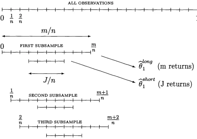
Our estimator of QVx makes use of the same principles as the TSRV estim ator in
Zhang et al. (2005a). We split the original sample of size n into K subsamples, with
the j th subsample containing rij observations. Introduce a constant (3and csuch th a t K = cnP. The dependence of K on n is suppressed in the sequel. For consistency
we will need (3> 1/2 — a. The optimal choice of (3is discussed in the next section.
By setting a = 0, we get the condition for consistency in Zhang et al. (2005a), th at (3> 1/2.5
Let \Y,Y]ni denote the j th subsample estim ator based on a if-spaced subsample of size rij,
T l j — l
K > T 3 = E ( y * * « - V . » * +j ) . 3 = 1. • • •,.K,
i= 1
and let
1 K
[ Y x r 9 = x ' E i Y x r * j=i
be the averaged subsample estimator. To simplify the notation, we assume th at n is divisible by K and hence the number of data points is the same across subsamples,
rii = n2 = ... = tik = n / K . Let n = n/ K .
Define the adjusted TSRV estim ator (jittered TSRV) as
Q V x = [V
v
]°”9
-
( ^ )
[y,r]{n}
. (i.5 )Compared to the TSRV estimator, this estimator does not involve any new parameters
th at would have to be chosen by the econometrician, so it is as easy to implement. The
need to adjust the TSRV estim ator arises from the fact th a t under our assumptions
TSRV is not always consistent. The problem arises due to end-of-sample effects
induced by heteroscedastic noise. For a simple example where the TSRV estimator
is inconsistent, let us simplify the model to the framework of Zhang et al. (2005a),
and introduce only heteroscedasticity in the noise, the exact form of which is to be
chosen below. Let us evaluate the asymptotic bias of TSRV estim ator.6
n V * E { Q v l SRV - Q V X ]
= n 1/6 |^ [ « , v\av9 — — E [u, «]nl + o (1)
= c - v ^ g ( 4 +* 4 +* + 4 4 )
2 = 1
- ( c - ' n - W - « - / “) g ( < , 4 , + 4 4 ) + 0 (1 ) 2 = 1
g ( 4 +4 +. + 4 4 ) - c' ln_1/2j F 4 4 + g 4 4 } + ° (
1)-2 = 1 V 2 = 2 i = n —K + l
We see th at the first and last K returns th at are ’’ignored” by averaged subsampled realized volatility [F, Y]avg ~ [u, u]avg have to be off-set by a fraction of the noise of all
returns, coming from [F, Y]n ~ [u, u]n. For this bias correction to work, the volatility
of the microstructure noise in the morning and afternoon has to be ’’close” to the volatility of the noise during the day. A simple counter-example th a t is motivated
by our empirical section 6.3 is a parabola on [0,1], u 2 ( i/ n ) — a + — 0.5) 2 /100, where a is any constant. In this case simple calculations give th a t TSRV estim ator is
inconsistent,
i /a —T S R V 1 i / c
n1/6E(QV"x - QVX ) = - ^ q ™176 + ° (1).
By contrast, jittered, R V , [Y, Y ]' mimics the structure of the volatility component
th at needs to be bias corrected for in [Y, Y]av9, which is
1 n —K
f
2 2 I 2 2\°ti+Keti+K U)tieti
and so delivers a consistent estim ator Q V X .
We remark th a t (1.5) is an additive bias correction and there is a nonzero proba
bility th at Q V x < 0. One can ensure positivity by replacing Q V X by max{QVx , 0},
but this is not very satisfactory. Note, however, th a t we usually have Q V x >
- r— T S R V
---Q V x (except for when first and last subsamples have all flat prices and so Q V x =
■^-~~~TSRV
---Q V x ), so the probability th at Q V x < 0 is lower th an the probability th a t
— T S R V
Q V X <0.
1.4
A sym p totic Properties
The expansion for [Y, Y]av9 and [Y, Y]n both contain terms due to the correlation between the measurement error and the latent returns. The main issues can be
illustrated using the expansion of \Y,Y]aV9 , conditional on the path of a t:
Sin
[Y, y ]°”» = QVx + 2^ J a tdt + E [u, «]“”9 + O K
(« ) (c )
(b)
(1.6)
where Z ~ iV (0 ,1 ), while the terms in curly braces are as follows: (a) the probability
limit of [X ,X ]avg, which we aim to estimate; (b) the bias due to correlation between the latent returns and the measurement error; (c) the bias due to measurement error;
(d) the variance due to discretization; (e) the variance due to measurement error.
Should we observe the latent price without measurement error, (a) and (d) would
an error of smaller order rC1!2. In the presence of the measurement error, however,
both [Y,Y]avg and [Y, Y]n are badly biased, the bias arising both from correlation
between the latent returns and the measurement error, and from the variance of the
measurement error. The largest term is (c), which satisfies
E [u, u]av9 = 2nn~a lu2 (u ) du + + O (n~a + n -1) = O (n n~a) ,
i.e., it is of order nn ~ a. So without further modifications, this is what [Y, Y \ av9
would be estimating. Should we be able to correct th at, the next term would be
2(5'yn/ K ) f &tdt arising from E [X, u]avg . This second term is zero, however, if there
is no correlation between the latent price and the MS noise, i.e., if 8 = 0. Interestingly
when we use the TSRV estim ator for bias correction of E [n, u]avg, we also cancel this second term.
The asymptotic distribution of our estimator arises as a combination of two effects,
measurement error and discretization effect. After correcting for the bias due to the
measurement error (terms like b and c in eqn. 1.6), we still have the variation due to the measurement error (term e in eqn. 1.6). We can see th a t its contribution to
the asymptotic distribution by observing how the estim ator converges to the realized
variance of the latent price X ,
— ( Q V x ~ [X, X ] avg^j = > iV
1
0,8£4 + 16 S2J
u 2 (u) du + 8J
u 4 (u ) gV o o
(1.7) The rate of convergence arises from vai[u,u]aV9 = O ( n / K n 2a). Both parts of the
noise u, which are v and e, contribute to the asymptotic variance. The first p art of
the asymptotic variance roughly arises from v a r^ , u ], the second part from var[v, e]
(which is nonzero even though the correlation between both term s is zero), and the
price, the first two terms disappear.
Should we observe the latent price without any error, we would still not know its
quadratic variation due to observing the latent price only at discrete time intervals.
This is another source of estimation error. Prom Theorem 3 in Zhang et al. (2005a)
we have
n x' 2 ([X, X ] avg - QVX ) =*► MTV ( 0, | J a ^ d t) , (1.8)
where M N ( 0 , S ) denotes a mixed normal distribution with conditional variance S
independent of the underlying normal random variable.
The final result is a combination of the two results (1.7) and (1.8), as well as
the fact th at they are asymptotically independent. The fastest rate of convergence
is achieved by choosing K so th a t the variance from the discretization is of the same order as the variance arising from the MS noise, so set n-1/ 2 = y / n / K n 2a. The result
ing optimal magnitude of K is such th at /? = 2 (1 — a ) / 3 . The rate of convergence
with this rule is n-1//2 = n _1/6_Q/3. The slowest rate of convergence is n -1/6, and it corresponds to large MS noise case, a = 0. The fastest rate of convergence is
n -1/3, which corresponds to a = 1/2 case. If we pick a larger (5 (and hence more
subsamples K ) th an optimal, the rate of convergence in (1.7) increases, and the rate
in (1.8) decreases and so dominates the final convergence result. In this case the final convergence is slower and only the first term due to discretization appears in the
asymptotic variance (see (1.9)). Conversely, if we pick a smaller /? (and hence K )
than optimal, we get a slower rate of convergence and only the second term in the asymptotic variance (’’measurement error” in (1.9)), which is due to the MS noise.
We obtain the asymptotic distribution of Q V x in the following theorem
T h e o re m 1.4.1. Suppose that { X u t € [0,1]} is a Brownian semimartingale satisfy
processes, independent of the process {W t, t E [0,1]}. Suppose further that the ob
served price arises as in (1.2) with a E [0,1/2). Let the measurement error uti be
generated by (1.3), with eti i.i.d. mean zero and variance one and independent of the
Gaussian process {W t , t E [0,1]} with E\eti\A+r} < 00 for some 7] > 0. Then,
(QVx - QVx) => N
(0,1),
d iscretiza tio n m easu rem en t erro r
Re m a r k s.
1. The quantity V(cr) collapses to the expression in Zhang et al. (2005a) when
cj(.) is constant.
2. If one could find a consistent estim ator V(<j) such th a t V( a) — V( a) = o(l) a.s., then the above theorem can be strengthened along the lines of Barndorff-Nielsen and
Shephard to a feasible CLT, i.e., V (a )~ l/ 2n l^2{QVx — Q V x) ==> N (0,1) from which
one could obtain confidence intervals for QVX . W ithout assuming S = 0 or constant
lu(.), the procedure of Zhang et al. (2005a), p. 1404, would work to estim ate V(a).
3. The main statem ent of the Theorem 1.4.1 can also be w ritten as
„ l / 6 + « / 3 ( g y x _ Q V x J ^ M N (Q) c V (< 7 )) f
where V{cr) = Vi (a) + with Vi(cr) being the discretization error, while M N
denotes a mixed normal distribution with conditional variance cV(a) independent of
the underlying normal random variable. We can use this to find the value of c th at
vided Vi(a) > 0, resulting in the asymptotic conditional variance (3/22/3)V21/^3V12^3(o‘). If one has consistent estimators Vj(a) — Vj(a) = o(l) a.s., j = 1,2, then Copt (a) =
(2V2(<7)/Vi((7))1/ 3 is consistent in the sense th a t copt(a) — c ^ c r ) = o(l) a.s.
4. Suppose now th a t the measurement error is smaller than above and we have a G [1/2,1) instead of a G [0,1/2). Then, there is a consistency condition /? >
1/3 th a t becomes binding and therefore optimal (3 allows the measurement error to
converge faster than the discretization error. For (3 = 1/3 + A (where A small and
positive) the rate of convergence is n-1/2 = n~^1~(3^ 2 = n_1//3+A/2 . Note th a t this is
exactly the rate th a t occurs when there is no measurement error at all. So choose (3G (1/3,1). The conclusion of the Theorem 1.4.1 becomes
V » - 1/ V 1- W2 ( Q V X - Q V x ) = * N ( 0 ,1 ) ,
where Vi(cr) = (4/3) f ajdt. This can be shown by minor adjustm ents to the proofs. 5. W hat if a > 1? This means th a t [u, u\ is of the same or smaller magnitude
than [X, X]. In the case a = 1 they are of the same order and identification breaks down. W hen a > 1, realized volatility of observed prices is a consistent estim ator of
quadratic variation of latent prices, as measurement error is of smaller order. This is
an artificial case and does not seem to appear in the real data.
How can we p ut this analysis in context? A useful benchmark for evaluation of the
asymptotic properties of nonparametric estim ators is the performance of param etric
estimators. Gloter and Jacod (2001) allow for the dependence of the variance of i.i.d. Gaussian measurement error pn on n and establish the Local Asymptotic Normality
(LAN) property of the likelihood, which is a precondition to asymptotic optimality
of the MLE. For the special case pn = p they obtain a convergence rate n -1/4, thus
allowing one to conclude th a t the MSRV and realized kernels can achieve the fastest
possible rate. They also show th a t the rate of convergence is u-1/ 2 if pn goes to zero
estim ator has a rate ti_1/3+a when there is no measurement error, which is also the
rate of convergence when the noise is sufficiently small. Also, Gloter and Jacod have
th a t for ” large” noise, the rate of convergence depends on the magnitude of the noise,
similarly to our results. The rate of convergence and the threshold for the magnitude
of the variance of the noise is different, though.
1.5
Sim ulation stu d y
In this section we explore the behavior of the estim ator (1.5) in finite samples. We
simulate the Heston (1993) model:
d X t = (nt - vt/2) dt + a tdWt
dvt = k, (0 — vt) dt + 7v\!2dBu
where vt = of, and Wt , B t are independent standard Brownian motions.
For the benchmark model, we take the param eters of Zhang et al. (2005a):
fj, = 0.05, « = 5, 0 = 0.04, 7 = 0.5. We set the length of the sample path to 23400 cor responding to the number of seconds in a business day, the tim e between observations
corresponding to one second when a year is one unit, and the number of replications
to be 100,000.7 We set a = 0. We choose the values of u and 5 so as to have a
homoscedastic measurement error with variance equal to 0.00052 (again from Zhang
et al. (2005a)), and correlation between the latent returns and the measurement error
7Note that in the theoretical part of the paper we had for brevity taken interval [0,1]. For the simulations we need the interval [0,1/250]. Suppose the parameter of interest is o \d t, the quadratic variation of X on [0,r]. In that case the asymptotic conditional variance of the Theorem 1.4.1 becomes
d u ^ .
This follows by simple adjustments in the proofs. We take r = 1/250.
V
T / T T
equal to —0.1. For this we use the identity
corr(AXti, A uti) = E{ a)
and the fact that for our volatility we have E (a) = 9, var(<r) = 6^2/ 2k,. We set /? = 2 (1 — a ) /3 . Figure 1.1 shows the common volatility path for all simulations.
8
7
6
5 4 3
20 0 .5 1 1.5 2 2 .5
[image:28.599.33.520.29.808.2]x 10
Figure 1.1: The common volatility path for all simulations.
First, we construct different models to see the effect of varying a and the number of observations within a day. We take the values of 6 and u th at arise from the benchmark model, and then do simulations for the following combinations of a and n. When interpreting the results, we should also take into account th at both of these parameters change the size of the variance of the measurement error. We measure the proximity of the finite sample distribution to the asymptotic distribution by the
the volatility path. Hence, we simulate the volatility path for the largest number
of observations, 23400, and perform all simulations using this one sample path of
volatility. The last param eter to choose is K , the number of subsamples. This is the
only param eter th at an econometrician has to choose in practice. We examine four
different values as follows (the expressions are all rounded to the closest integer):
( 2 V r2 / l / 1 ) 1/ 3 n 3 ( 1 - “ ) asymptotically optimal rate and c Tables A .l and A .2 ^ g ( l - a ) variation of above
Tables A .S and A. 4
2
77,3 variation of above Table A .5
( 1 £ ) 1 / 3 " 1 / 3 Bandi and Russell (2006a, eq. 24) Table A .6
Table 1.1: Choices of K
Table A .l contains the interquartile range errors (IQRs), in per cent, with the
asymptotically optimal rate and constant (in terms of minimizing asymptotic mean squared error) for K . T hat is, we use K = {2V2/V1) 1/37t,2(1—"I/3, rounded to the nearest
integer, where V\ and V2 are discretization and measurement errors from (1.9). Table
A.2 contains the values of K .
First of all, for small values of a , the percentage errors decrease with n as predicted
by the theory. However, we do see some large errors, and from the values of K in
Table A.2 we can guess this is due to the asymptotically optim al rule selecting very
low 0^ • In fact, for the volatility path used here, = (2V2/V1)1/ 3 = 0.0242. Hence,
another experiment we consider is an arbitrary choice c = 1. The next two tables
(Table A.3 and A.4) contain the percentage errors and values of K th a t result from using K = n 2(1-a)/3.
The performance of this choice is much better. We can see from Table A.3 th a t
for small values of a, the asymptotic approximation improves with sample size. The
sign of the error changes as a increases for given n, meaning th a t the actual IQR is
below th at predicted by the asymptotic distribution for small a and small n but this
Another variant th a t does not include the unobservable a would be to use K =
n 2' 3.
Finally, we consider a method proposed by Bandi and Russell (2006a), which
requires some discussion. They establish the exact mean squared error of TSRV
under the assumptions of the independent additive noise model, and in addition they
u 1
assume asymptotically constant volatility, i.e., f o \d u — f a ^d u /n for each i, as
U-i o
well as E (e4) = 3E 2 (e2). Two assumptions are not satisfied in our simulation setup, the independence between the noise and the latent returns, as well as the assumption
u l
f credit, = f o 2ud u /n for each i (see Figure 1.1). Therefore, this should be considered
ti— i 0
as another ad hoc selection method in our simulation setup. We note th a t this
bandw idth choice results in an inconsistent estim ator in our framework and in the
framework of ZMA (2005a) (i.e., when a = 0, ^ > 1/2 is required for consistency). Note th a t the choice K was derived for Q V without jittering, but this
end-of-sample adjustm ent, though theoretically crucial, is negligible in simulations and, as we
will see in the next section, also in real data. Table A.6 contains the IQR percentage errors and values of K th a t result from using K BR = (3 R V 2/2 R Q )1^3 n 1/3, where
R V is the realized variance, R V = (A^zoiu)2 and RQ is the realized quarticity,
RQ = § $3 (AYiow)4. Here, Y ^ is low frequency (15 minute) returns, which gives S = 24 to be the number of low frequency observations during one day.
We see th a t the IQR errors of this choice get worse with sample size for small
a , which reflects the inconsistency predicted by the theory. On the other hand the
errors are small and improve with n for large a , i.e., when the noise is small. The
performance is generally better than with asymptotically optimal K, except for cases
th a t have bo th large n and small a , including the case a = 0 usually considered in
the literature. We notice th a t K BR rule gives better results th an the asymptotically
optimal rule when it chooses a larger K, which is in most cases, but not all. In
the performance of this choice is still disappointing, especially for small a. We con
clude th at in this setting the K BR rule is not always the best choice according to our
criterion.
It has been noted elsewhere th a t the asymptotic approximation can perform
poorly, see Gongalves and Meddahi (2005) and Ai’t-Sahalia, Zhang and Mykland (2005a).
From Tables A .l, A.3, and A.5 we see th at magnitude of noise does not affect the quality of the asymptotic approximation. Although we see the interquartile range
error having some relationship with a in Table A.3 and especially Table A .l, this is
purely driven by changes in K . This is evidenced by Table A.5 where the rule for K does not depend on a and the respective error is close to constant for the same
number of observations and different a. Another conclusion here is th a t a good rule
for K does not necessarily have to depend on a , which is convenient for practical purposes.
In a second set of experiments we investigate the effect of varying cj, which controls the variance of the second part of the measurement error, for the largest sample size.
Denoting by uj\ the value of u 2 in the benchmark model, we construct models with
cj2 = uj2, Aw2, 8lu2, IOo;^, and 20u 2. The corresponding interquartile errors are 0.96%, 1.26%, 1.93%, 2.29%, and 4.64%.
In a third set of experiments we investigate the effect of varying 5, which controls
the size of the correlation of the latent returns and measurement error. Denoting
by S\ the value of S2 in the benchmark model, we construct models with S2 being
from 0.01 x S2 to 20 x S2. The exact values of S2, as well as corresponding correlation
between returns and increments of the noise, and the resulting interquartile errors are
reported in Table A. 7. We can see th a t when the number of observations is 23400,
there is no strong effect from the correlation of the latent returns and measurement
1.6
Em pirical analysis
To illustrate the above ideas, we perform a small empirical analysis. We discuss es
tim ation of a, <*;(.), and the quadratic variation of the latent price. The endogeneity
param eter 5 is unfortunately nonparametrically unidentified and so cannot be esti
mated. Its sole purpose is in allowing for flexible size and sign of endogeneity, with
respect to which our estim ator of quadratic variation is robust.
Figure A .l in the appendix shows the volatility signature of the d ata we use, which
is IBM transaction data, year 2005. The plot indicates th a t market microstructure
noise is prevalent at the frequencies of 10 —15 minutes and higher. Since the volatility
signature plot does not become negative, one cannot find evidence of endogeneity
using the method of HL (2006). As pointed out already by HL(2006), this does not mean there is no endogeneity.
1.6.1 T he D a ta
We use IBM transactions d ata for the whole year 2005. We employ the d ata cleaning
procedure as in HL (2006), main paper and rejoinder. First, we use transactions from NYSE exchange only as this is the main exchange for IBM. Second, we use only
transactions from 9:30AM to 4:00PM. Third, for transactions with the same time
stamp, we use the average price. Fourth, we remove outliers as follows. If the price
is too much above the ask price or too much below the bid, we remove it. Too high
means more than spread above the ask, and too low means more than spread below
the bid. Fifth, we remove days with less than 5 hours of trading (there were none).
For discussion of the advantages of this procedure see HL (2006). The mean number
of transactions per day in our cleaned d ata set is 4,484 (for comparison, there are
1.6.2
E stim ation o f
a
The param eter th a t governs the magnitude of the m icrostructure noise, a, can be
consistently estimated. Recall th at the leading term of realized volatility [Y, Y]n is
[it, u]n i.e.,
[Y, Y]n = y > tj+1 - + o ^ n 1-*) i=1
n—1
= n ° y ^ ( a iti+1et,+1 - wtiet i + 5\/n(W ,,+1 - Wt())2 + Opin1 a) i=1
= n 1~ac + op(n l~a)
for some positive constant c. It follows th at
logQY, Y]n/n ) = —a log n + log c + op(\og n).
We therefore estimate a by
log ( [ O T / n ) n i m
a = ---— r—--- , (1.10)
log(n)
see Linton and Kalnina (2007).
Although this is a consistent estimator for a, it has a bias th a t decays slowly. To
reduce the bias, we estim ate a over windows of 60 days instead of 1 day, i.e., we take
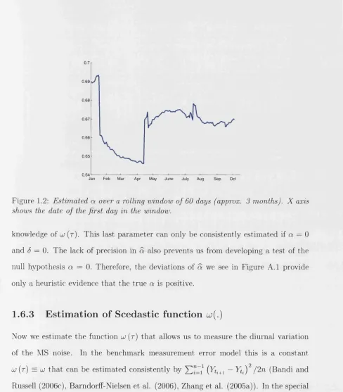
our fixed interval [0,1] to represent 3 months instead of 1 day. Figure 1.2 shows the
estimates over the whole year 2005 where we roll the 60 day window by 1 day. We
see th at a varies between 0.64 and 0.7 with an average value of 0.67.
Although this is a consistent estimator for a , it is not precise enough to give
a consistent estim ator of n a . As a consequence, this estim ator cannot be used for
consistent inference for Q V X. In Linton and Kalnina (2005) we provide a sharper bias
0.7
0.69
A
0.68
0.65 0.67
0.66
0.64
J a n F e b Mar Apr May J u n e July Aug S e p Oct
Figure 1.2: Estimated a over a rolling window of 60 days (approx. 3 months). X axis shows the date of the first day in the window.
knowledge of u (r). This last parameter can only be consistently estimated if a = 0 and (5 = 0. The lack of precision in a also prevents us from developing a test of the null hypothesis a = 0. Therefore, the deviations of a we see in Figure A .l provide only a heuristic evidence that the true a is positive.
1.6.3
E s tim a tio n o f S ce d a stic fu n c tio n
u j{ . )Now we estimate the function u (r) that allows us to measure the diurnal variation
of the MS noise. In the benchmark measurement error model this is a constant
lj ( t ) = uj th at can be estimated consistently by {^U+i “ ^t*)2 / ^ n (Bandi and
Russell (2006c), Barndorff-Nielsen et al. (2006), Zhang et al. (2005a)). In the special case a = 0 and (5 = 0 this estimator would converge asymptotically to the integrated variance of the MS noise, f u 2(r) dr. We can estimate the function J 1 (.) at a specific point t using a simple generalization of the approach of Kristensen (2006) to the case
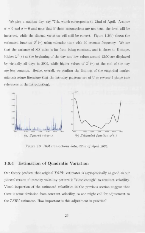
[image:34.600.29.517.33.590.2]We pick a random day, say 77th, which corresponds to 22nd of April. Assume a = 0 and <5 = 0 and note that if these assumptions are not true, the level will be incorrect, while the diurnal variation will still be correct. Figure 1.3(b) shows the
estimated function Q2 (r) using calendar time with 30 seconds frequency. We see that the variance of MS noise is far from being constant, and is closer to U-shape. Higher u)2 (r) at the beginning of the day and low values around 13:00 are displayed by virtually all days in 2005, while higher values of uj2 (r) at the end of the day
are less common. Hence, overall, we confirm the findings of the empirical market
microstructure literature th at the intraday patterns are of U or reverse J shape (see references in the introduction).
0.06r 0.05 0.04 0.03
0.02 ,
9:30 11:00 12:00 13:00 14:00 15:00 16:00
(a) Squared returns
Figure 1.3: IBM transactions data, 22nd of April 2005.
1 .6.4
E s tim a tio n o f Q u ad ratic V a ria tio n
Our theory predicts th at original T S R V estimator is asymptotically as good as our jittered version if intraday volatility pattern is ’’close enough” to constant volatility. Visual inspection of the estimated volatilities in the previous section suggest th at there is some deviation from constant volatility, so one might call for adjustment to
the T S R V estimator. How important is this adjustment in practice?
(b) Estimated function uj2(.)
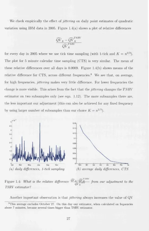
[image:35.600.31.518.42.825.2]We check empirically the effect of jittering on daily point estimates of quadratic variation using IBM data in 2005. Figure 1.4(a) shows a plot of relative differences
— T S R V
Q V x - Q
T S R V
Q V x
for every day in 2005 where we use tick time sampling (with 1-tick and K = n 2/3).
The plot for 5 minute calendar time sampling (CTS) is very similar. The mean of these relative differences over all days is 0.0009. Figure 1.4(b) shows means of the relative difference for CTS, across different frequencies.8 We see that, on average, for high frequencies, jittering makes very little difference. For lower frequencies the change is more visible. This arises from the fact th at the jittering changes the T S R V estimator on two subsamples only (see eqn. 1.12). The more subsamples there are, the less important our adjustment (this can also be achieved for any fixed frequency by using larger number of subsamples than our choice K = n 2/3).
Mar May July Sep Nov
(a) daily differences, 1-tick sampling
0.16 0.14 0 12 0.08 0 06 0.04
0.02
10m 8m 6m 4m 2m 45s 15s 5s
(b) average daily differences, CTS
- T S R V
Figure 1.4: What is the relative difference — from our adjustment to the QV x
TSRV estimator?
Another important observation is that jittering always increases the value of QV
[image:36.600.30.520.46.807.2]estimates, since we can write
QVT
x
RY = QV
x
+ \ (
y
, {Yti+1
-
Ytl)2
+
J2
(y‘<+. - y*.)2) >
QVx-
(1-12)\ i= 1 i —n —K + 1 )
The more there is variation in the beginning of the day and the end of the day, the
larger is the adjustm ent. This implies th at jittering partly alleviates the problem
th a t the usual TSRV estim ator can sometimes become negative. W ith our d ata set,
the only negative value (though very small) we saw was on February 28 when we
calculated TSRV estim ator with 10 minutes CTS frequency. The jittered version was positive.
We conclude th a t for most applications our estim ator is very close to the T S R V
estimator, and so for practical applications plain T S R V estim ator can be used, with
out adjustm ent for heteroscedastic market microstructure noise. As a result, as far as point estimates are concerned, the existing empirical studies of T S R V estimator are
still valid in our theoretical framework. See, for example, investigations of forecasting performance in A'lt-Sahalia and Mancini (2006), Andersen, Bollerslev, and Meddahi
(2006), Bandi, Russell, and Yang (2007), and Ghysels and Sinko (2006).
1.7
C onclusions and E xtensions
In this paper we showed th a t the TSRV estim ator is consistent for the quadratic
variation of the latent (log) price process when the measurement error is correlated
with the latent price, although some adjustm ent is necessary when the measurement
error is heteroscedastic. We also showed how the rate of convergence of the estim ator
depends on the m agnitude of the measurement error.
Inference for TSRV estim ator is robust to endogeneity of the measurement error.
Provided the suggested adjustm ent to the estim ator is implemented to preserve con
rate of convergence depends on the magnitude of the noise, inference is not robust to
possible deviations from assumptions about this magnitude. We plan to investigate
this question further.
Other examples where inference question needs to be solved include autocorre
lation in measurement error (as in A'lt-Sahalia, Mykland, and Zhang, 2006a), or
other generalizations to the independent additive error model (Li and Mykland 2007). Gongalves and Meddahi (2005) have recently proposed a bootstrap methodology for
conducting inference under the assumption of no noise and shown th a t it has good
small sample performance in their model. Zhang, Mykland, and Ait-Sahalia (2005b)
have developed Edgeworth expansions for the TSRV estimator, and it would be very
interesting to use this for analysis of inference using bootstrap. The results we have
C hapter 2
Subsam pling H igh Frequency D a ta
2.1
Introduction
This paper proposes the first autom ated m ethod for conducting inference with high frequency data. In particular, it proposes to estim ate the asymptotic variance of
some estimator without relying on the exact expression of the asymptotic variance.
In the traditional stationary time series framework, this task can be accomplished by bootstrap and subsampling variance estimators, b ut these are inconsistent with high
frequency data.
A new subsampling method is developed, which enables to conduct inference for
a general class of estimators th a t includes many estimators of integrated volatility.
The question of inference on volatility estimates is im portant due to volatility being
unobservable. For example, one might want to test whether volatility is the same on
two different days, or in two different time periods within the same day. The latter
corresponds to testing for diurnal variation in the volatility. Also, a common way
of testing for jumps in prices is to compare two different volatility estimates, which
converge to the same quantity under the null hypothesis of no jumps, but are different
inferential method is needed to determine whether the two volatility estimates are
significantly different.
To illustrate the robustness of the new method, this paper considers the example of
inference problem for the integrated variance estim ator of Ait-Sahalia et al. (2006a),
in the presence of market microstructure noise. As several assumptions about the
market microstructure noise are relaxed, the expression for the asymptotic variance
becomes more complicated, and it becomes more challenging to estim ate each com
ponent of the variance separately. On the other hand, the new subsampling method
delivers consistent confidence intervals th at are simple to calculate.
According to the fundamental theorem of asset pricing (see Delbaen and Schacher-
mayer, 1994), the price process should follow a semimartingale. In this model, in tegrated variance (sometimes called integrated volatility) is a natural measure of
variability of the price path (see, e.g. Andersen, Bollerslev, Diebold, and Labys,
2001). W ith moderate frequency data, say 5 or 15 minute data, this can be es
tim ated by the so called Realized Variance (RV), a sum of squared returns. The nonparametric nature of Realized Variance and the simplicity of its calculation have made it popular among practitioners. It has been used for asset allocation (Fleming,
Kirby, and Ostdiek, 2003), forecasting of Value at Risk (Giot and Laurent, 2004),
evaluation of volatility forecasting models (Andersen and Bollerslev, 1998), and other
purposes. The Chicago Board Options Exchange (CBOE) started trading S&P 500
Three-Month Realized Volatility options on October 21, 2008. Over the counter,
these and other derivatives w ritten on RV have been traded for several years. These
financial products allow one to bet on the direction of the volatility, or to hedge
against exposure to volatility. Pricing of these derivatives is done according to the
Suppose the log-price X t follows a Brownian semimartingale process,
d X t = [itdt + atdWt , (2.1)
where 11, a, and W are the drift, volatility, and Brownian Motion processes, respec
tively. Our interest is in estim ating volatility over some interval, say one day, which
we normalize to be [0,1]. The quantity of interest is captured by integrated variance, or quadratic variation over the interval, which is defined as
IV X = j aids. Jo
Realized variance (or empirical quadratic variation) is a consistent estim ator of inte grated variance in infill asymptotics, i.e., when the the approximation is made as the
time distance between adjacent observations shrinks to zero. According to this ap
proximation, therefore, the estimation error in RV should be smaller for even higher frequency d a ta th an 5 minutes. Ironically, this is not the case in practice. For the
highest frequencies, the d ata is more and more clearly affected by the bid-ask spread and other market m icrostructure frictions, rendering the semimartingale model inap
plicable and RV inconsistent. Zhou (1996) proposed to model high frequency d ata as
a Brownian semimartingale with an additive measurement error. This model can rec
oncile the main stylized facts of prices both in moderate and high frequencies. Zhang,
Mykland, and A'it-Sahalia (2005) were the first to propose a consistent estim ator of
integrated variance in this model, in the presence of i.i.d. m icrostructure noise, which
they named the Two Scale Realized Volatility estimator. Consistent estimators in
this framework were also proposed by Barndorff-Nielsen, Hansen, Lunde, and Shep
hard (2008a), Christensen, Oomen, and Podolskij (2008), Christensen, Podolskij, and
Vetter (2006), and Jacod, Li, Mykland, Podolskij, and Vetter (2007). Ai't-Sahalia,
the case of stationary autocorrelated microstructure noise, but do not propose an in