Modelling the Dynamic Behaviour of the Wheel Rail Interface by Using a Novel 3D Wheel Rail Contact Model

University of Huddersfield Repository

Anyakwo, Arthur, Pislaru, Crinela, Ball, Andrew and Fengshou, Gu

Modelling the Dynamic Behaviour of the Wheel­Rail Interface by Using a Novel 3D Wheel­Rail 

Contact Model

Original Citation

Anyakwo, Arthur, Pislaru, Crinela, Ball, Andrew and Fengshou, Gu (2011) Modelling the Dynamic 

Behaviour of the Wheel­Rail Interface by Using a Novel 3D Wheel­Rail Contact Model. In: 5th IET 

Conference on Railway Condition Monitoring and Non­Destructive Testing (RCM 2011), 29­30 

November 2011, Derby Conference Centre, UK. 

This version is available at http://eprints.hud.ac.uk/id/eprint/13466/

The University Repository is a digital collection of the research output of the

University, available on Open Access. Copyright and Moral Rights for the items

on this site are retained by the individual author and/or other copyright owners.

Users may access full items free of charge; copies of full text items generally

can be reproduced, displayed or performed and given to third parties in any

format or medium for personal research or study, educational or not­for­profit

purposes without prior permission or charge, provided:

•

The authors, title and full bibliographic details is credited in any copy;

•

A hyperlink and/or URL is included for the original metadata page; and

•

The content is not changed in any way.

For more information, including our policy and submission procedure, please

contact the Repository Team at: E.mailbox@hud.ac.uk.

MODELING THE DYNAMIC BEHAVIOUR OF THE WHEEL

RAIL INTERFACE USING A NOVEL 3D WHEEL-RAIL

CONTACT MODEL

A. Anyakwo*, C. Pislaru, A. Ball, F. Gu

*Diagnostic Engineering Research Centre, University of Huddersfield, U.K, Email: arthur.anyakwo@hud.ac.uk

Keywords: multibody modelling, wheel-rail interface, wheel

profiles, vehicle dynamics, condition monitoring

Abstract

Methods for multibody modelling and simulation should accurately replicate the dynamic behaviour of rail-wheel interface including precise values for wheel-rail contact positions. This paper studies the development of a novel 3-D wheel-rail contact model which is used for dynamic simulation of a suspended wheelset with parameters listed for a typical Mark IV coach. The contact point locations on the wheel and rail are determined by the minimum difference method considering the lateral displacement, yaw angle and the roll angle. The proposed new 3D wheel-rail contact model can be applied in railway condition monitoring techniques to estimate the wheel geometry parameters and thus to achieve practical optimised wheel-rail interfaces.

1

Introduction

The dynamic behaviour of railway vehicle on the track is influenced by wheel-rail interaction. Any slight deviation in the shape of the wheel and rail profiles affects the movement of the vehicle on the track. The implementation of a comprehensive rail vehicle dynamic model in the multibody simulation software package requires the location of all contact points on the wheel-rail contact. Two dimensional wheel-rail contact models are limited to the two dimensional motion of the two surfaces and are thus not very suitable for application in steep rail track curves where the yaw angles are large. Wickers [1] applied 2D wheel-rail contact method to calculate the wheel-rail contact coordinates considering the lateral displacement and the roll angle as inputs. Also the 2D wheel-rail contact method was used to design the wheel profiles considering the contact angle function [2] or the rolling radius difference function [3].

The lateral displacement, roll angle and the yaw angle are used to depict the movement of the wheelset on the track in three dimensions. Two methods used for 3-D wheel-rail contact are rigid contact method and semi-elastic method. The rigid contact method [4,5] comprises a set of algebraic nonlinear differential equations used to describe the dynamics of the wheel-rail contact in 3D. Indentation and lift are not considered due to the fact that the wheel movement is made up of five degrees of freedom (DOF) with respect to the rail. The semi-elastic methods allow the management of multiple contact points and are generally used for automotive and

railway applications [5, 6]. The wheel is assumed to have six DOF with respect to the rail. The normal contact forces acting on the wheel-rail contact are defined as a function of indentation using Hertz theory for two surfaces in contact. They require look-up tables with the values of the wheel-rail co-ordinates depending on the lateral displacement, yaw and roll angles. The number of simulated contact points is limited so the management of multiple contact points is hard to achieve.

2 Development of mathematical 3D wheel-rail

contact model

Generative functions for P8 wheel profiles and BS 113A rail profile are applied as inputs. The contact position locations on the wheelset and rail are obtained by using the piecewise cubic interpolation polynomial and the calculated lateral displacement, roll angle and yaw angle (their initial values are assumed to be zero). The variation between the wheelset and rail positions is applied to the minimum difference method algorithm. The rolling radius difference function and the contact angle function are determined when the indentation is negative. The block ‘Normal contact problem’ (see Fig. 1) represents the calculation of the normal contact forces and contact patch dimensions by using Hertz theory. These values and the rolling radii of left and right wheel functions are used to evaluate the tangential contact forces. These calculated values and the primary suspension parameters corresponding to BR MK IV coach [11] are included in the differential equations describing the wheelset dynamic behaviour. The equations are solved using Runge-Kutta method.

Fig. 1 Development of 3D Wheel-rail contact model

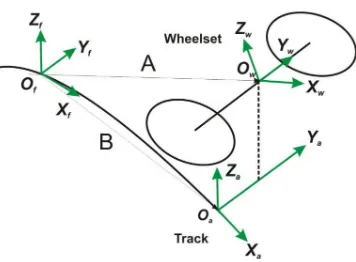
2.1 Reference Frame Definitions for the Track

Three frames of reference are used to define wheel-rail contact geometry. They include the fixed reference frame, the auxiliary reference frame and the local reference frame. The track reference frames are shown in Fig. 2.

. The fixed reference system (Of, Xf, Yf, Zf) defines the track

as a three dimensional curve. The auxiliary reference system (Oa,Xa,Ya,Za) follows the wheelset during program

simulations. It is defined on the rail tracks. The Xa axis is

tangential to the track centreline in the longitudinal direction of point Oa. Ya is the lateral direction with respect to the rail

plane while Za is in the normal direction with respect to the

plane of the rail.

The unit normal vectors obtained from the auxiliary system can be defined as follows;

i k = i k A (1)

where Acant is the rotation matrix defined as a function of the

cant angle β. The cant angle for the rail is 1/20 radians

Fig. 2 Reference frames for the wheel-rail contact model

The unit normal vectors obtained from the auxiliary system can be defined as follows [8, 9];

i k = i k A (1)

where Acant is the rotation matrix defined as a function of the

cant angle β. The cant angle for the rail is 1/20 radians

A β =

1 0 0

0 cosβ −sinβ

0 sinβ cosβ

(2)

The local reference system in Ow,Xw,Yw,Zw is defined

whereby Yw is rigidly fixed to the wheelset axle. The origin of

the wheelset Ow corresponds with the centre of gravity G of

the wheelset. Let V and V represent the position of a point in the auxiliary and reference local frame respectively, then the kinematic equation is generally expressed as follows:

= O + A V (3)

where O is the wheelset centre coordinates of mass expressed with respect to the auxiliary system and A is a function of the yaw angle ψ and the roll angle φ.

= !cos -sinsin cosψψcoscosφφ −cossinψψsinsinφφ

0 sinφ cosφ

$ (4)

O = %0&

%'

(5)

where %_& and %_' are the lateral and vertical displacement of the wheelset respectively.

In the local reference system the wheelset function is derived by a generative function that represents half of the wheelset axle. The generative profile of the wheelset ( ) with P8 wheel profiles on each wheel is shown in Fig. 3.

The position of a point on the axle local reference frame can be represented as follows

* , ) = ! *)

−,( ) − *

Fig. 3 Wheelset generative function

Similarly, the position of the same generic point on the wheelset with respect to the auxiliary reference system is;

* , ) = . + * , ) = !/0

1 $ (7)

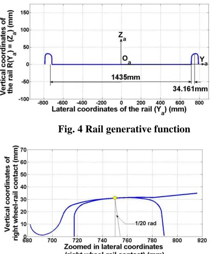
The generative rail function is plotted in Fig. 4 with BS 113A rail profiles on both rails. Also a zoomed in portion of the wheel-rail profile is shown in Fig. 5.

Fig. 4 Rail generative function

Fig. 5 Zoom-in portions for right BS 113A and P8 profile

In the auxiliary system, the coordinates of the point on the rail can be expressed as:

* , ) = *)

2 ) (8)

2.2 Minimum Difference Method

The minimum difference method is used in order to simplify and further improve the computational burden associated with the minimum distance method. The main motivation for using

this method is that the contact points in the wheel and rail surfaces minimize the difference between the wheel-rail contacts in the direction of the unit normal vector Ca.

Fig. 6 Minimum difference (right wheel-rail contact)

The minimum difference method definition is illustrated in Fig. 7 where C = and D =

3 * , ) = * , ) − * , ) . 5 (9)

Where * , ) = !

/ 0

6 0 $ (10)

For each wheel-rail contact the difference 3 * , ) is a function of two variables * and ) . The contact points can thus be found by solving synchronously for the two variables using numerical optimization technique such as Simplex method. For real-time simulations it is preferable to reduce Equation (9) to one dimensional form in one variable ) which can easily be solved numerically. Introducing the definitions of the contact positions for the wheel and the rail in the respective frames in Equation (9) it yields [8,9];

3 * , ) = %'+ 78. * , ) − 2 %&+ 7 . * , )

(11) Where a11 to a33 is equivalent to the rotation matrix variables

defined in Equation (5) and 7₉:, 7: and 7₈: are the transpose of the row vectors of column [A2].

!79

:

7:

78:

$ = 77999 779 77988

0 78 788

(12)

Taking the partial derivatives of Equation (11) with respect to the variables * , ) , that _;=;<

> and

;<

;?> and equating it to

zero we will have two different representative equations. Carrying out further reductions of these equations leads to a quadratic solution of the variable * with two roots. Substituting the roots of the quadratic equation * as a function of ) and substituting into the second component of the partial derivative of the difference, we have that the following expression

Equation (13) has now been reduced to a simple equation with variable ) ranging from (692 ≤) ≤ 815) mm for the right wheel-rail contact geometry part and from (-815 ≤−) ≤ -692) mm for the left wheel-rail contact geometry. The equation has two real values of * and ) corresponding to the twenty-one specified numerical points. The solution of the variables must satisfy Equation (13). The following indentation condition must be considered:

AB= 3B. C B ≤ 0 (14)

Note that from Equation (11) the vertical displacement uz

adds to the difference equation. Taking the partial derivatives of Equation (11) eliminates uz. Hence the only parameters

used in determining minimum of the contact points depend on three variables; φ roll angle, yaw angle ψ and lateral displacement uy. (see Table 1)

Input parameter

Range Step

φ (rad) -0.01 – 0.01 0.0005

ψ (rad) -0.01 – 0.01 0.0005

uy (mm) -10 – 10 0.5

Table 1 Parameters for wheelset degree of freedom

The rolling radius difference function can be obtained from the numerical simulations by substituting the values of variables * , ) into Equation (7). The constant uz from

the wheel-rail geometry description in Fig. 3 and Fig. 4 is 491mm. Extracting the third component of Equation (7) in the vertical direction and subtracting the results obtained from the nominal rolling radius given for the simulation as 460 mm, the rolling radius difference is realized in Fig. 8. For simulation purposes, a look-up table showing the rolling radius difference function and the contact angle function which is a function is shown below. A distance of 0.5 mm spacing was chosen and then piecewise cubic interpolation was used to interpolate between the functions described. From the simulations carried out for the BS 113A profile and P8 wheel profile, 0.5 mm increments was sufficient enough to carry out dynamic simulations. Due to the conformal nature of the P8 profile the contact angle function [2] derived was found by substituting values of the lateral co-ordinate function into the derivative of the wheelset generative function as follows

E = 7FGH7C I_J?J-_>K (15)

The rolling radius difference function and the contact angle function is shown in Fig. 4 and Fig. 5. Note that since the wheelset is symmetrical, hence the same calculation for the contact angle occurs at the left wheel-rail contact where the lateral co-ordinate ) is negative.

2.3 Normal contact problem

The normal contact forces [12] acting on the wheel-rail contact patch depend on the axle load, wheelset mass and

contact angle. The wheelset is assumed to be on a straight track with the axle load (Wload) of 110kN. The mass (m) of

the wheelset is based on parameters for the British MK IV vehicle [11]. The roll angle has very little effect on the contact angle function since the values are really small and they depend on the rolling radius difference function.

Fig. 7 Rolling radius difference function

Fig. 8 Contact angle function (Right wheel-rail contact)

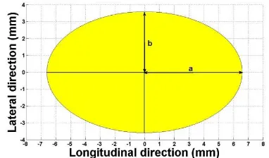
Anyakwo et al [12] determined the normal contact forces acting on the wheel-rail contact patch. These forces are used to estimate the contact patch size dimensions based on Hertz contact theory [4]. The simulated values for the wheel-rail contact patch dimensions considering the wheelset in central position is shown in Fig. 9.

Fig. 9 Wheel-rail contact patch at central position

2 = I_MNO L_θK (16)

Where Rx is the longitudinal radius of curvature of the wheel

and Ris the rolling radius of the left and right wheel-rail contact [14]. The normal contact pressure acting on the contact patch is semi-ellipsoidal in shape with maximum contact pressure occuring at the centre of the elliptical contact patch. It can be calculated as thus;

P = 8Q_R S1 − I K − I&K TU.V (17)

Where x and y are the co-ordinates of the wheel-rail contact patch in the longitudinal and lateral directions respectively and N is the normal contact force.

2.3 Tangential Contact Problem

The tangential contact problem involves calculating the creep forces that are developed in the wheel-rail interface as a result of braking, traction and acceleration. The creepages (lateral, longitudinal and spin) are used to calculate the creep forces acting on the contact patch using Kalker’s linear coefficient tables [15]. The creepages for a dynamic wheel-rail contact can be calculated as follows;

Lateral creepage (right/left wheel-rail contact)

W =_XJJ& −ψ (18)

Longitudinal creepage

WY Z [BZ\ = −_XJWJψ−λ_L&_] (19)

WY Z W^_ = −_XJWJψ+λ_L&_] (20)

Spin creepage

`aB [BZ\ = −_Lλ_]−_XJJψ (21)

`aB W^_ =_Lλ_]−_XJJψ (22)

Where λ is the effective conicity of the wheel profile. For

new P8 wheel profile the equivalent conicity is non-linear due to the wheel profile design. The effective conicity can be expressed as a function of the lateral displacement and can be calculated as follows;

λ 0 =LL<_& (23)

Where RRD is the rolling radius difference function expressed as;

RRD(y) = 2_[ 0 − 2_W 0 (24)

Rr and Rl represent the rolling radius of the right wheel and

left wheel-rail contact respectively and y is the lateral displacement. V is the forward velocity of the wheelset and R0

is the nominal rolling radius difference.

The creep forces are determined using Kalker’s theory. For small creepage values, the creep force/creepage ratio is linear. This implies that the creep forces increase linearly as the

creepage increases. For large creepages, the creep forces must be limited by applying Coulomb’s maximal saturation law. At this region the creep/creepage ratio is highly non-linear. This occurs at flange contact. Kalker’s linear theory calculation at the saturation region is generally linear. Heuristic non-linear creep force model can be used to calculate the limiting values that occur at the wheel-rail contact patch in this case. The saturation constant d [13] is used to limit the creep forces calculated via Kalker’s contact theory:

b = c

9

ηdIη−

9 8η +

9

eη8Kf η≤ 3 9

η, η> 3

i (25)

where

η= Sjk lmk&ln ].o

pq T (26)

where µ represents the coefficient of friction (0.3) and N is the normal contact force acting on the contact patch. η is the unlimited normalized creep force ratio while Fx and Fy are the

longitudinal and lateral creep forces developed at the wheel-rail interface. Normalized re-calculated creep forces at the saturation region can be defined as thus:

r = br (27)

r& = br& (28)

s' = bs' (29) where Fx, Fy represent the longitudinal, lateral creep forces.

Mz is the spin creep moment. All the creep forces depend on

the Kalker’s linear creep coefficient, shear modulus of rigidity and Kalker’s linear coefficients [12].

2.4 Wheelset dynamic behaviour

The wheelset dynamic behaviour of a straight track can be investigated by summing all the creep forces and normal contact forces generated at the wheel-rail contact patch. The summation of the total creep forces plus the forces generated as a result of longitudinal shift variation of the wheelset as it moves on the track [13]. Details of calculation of the normal contact vertical forces and moments as a result of the longitudinal variation can be found in [12]. For simulation purposes the following parameters based on British Mark IV coach is displayed in [11], [13]. The suspended parameters used for the simulation can be found in [13].

3 Numerical Simulation results

The two degree of freedom differential equations are solved using numerical differentiation. Runge Kutta’s fourth other method was used to solve the equations for initial value inputs of the lateral displacement and the yaw angle. Initial input parameter for the lateral displacement is given as y = 7.5mm thats just at flange contact. The yaw angle input variable from the wheelset geometry is given as 0.00125 radians.

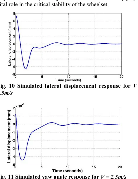
the suspended wheelset on the track shows that the wheelset stabilized after 15 second for both lateral displacement and yaw angle as shown in Fig. 10 and Fig. 11. The wavy sinusoidal response of the wheelset for a given lateral displacement and yaw angle indicates that the conicity plays a vital role in the critical stability of the wheelset.

Fig. 10 Simulated lateral displacement response for V =

2.5m/s

Fig. 11 Simulated yaw angle response for V = 2.5m/s

The non-linear conicity function in Equation (23) was used to for dynamic analysis. For an improved dynamic response of the single wheelset, the conicity function needs to be linearized to obtain the equivalent conicity function. Several methods exist in literature for linearizing the conicity function. In this paper, the main motivation was towards simulating the dynamic behaviour of the track. Future work would concentrate on obtaining the equivalent conicity function that would be used for railway vehicle dynamic simulations and for condition monitoring applications where the wheel profile parameters and the forces could be estimated.

4

Conclusions

This paper studies the development of a novel 3-D wheel-rail contact model which is used for dynamic simulation of a suspended wheelset with parameters listed for a typical Mark IV coach. The contact point locations on the wheel and rail are determined by the minimum difference method considering the lateral displacement, yaw angle and the roll angle. The proposed new 3D wheel-rail contact model accurately replicate the dynamic behaviour of rail-wheel interface and can be employed in railway condition monitoring techniques to estimate the wheel geometry parameters and achieve optimised wheel-rail interfaces

References

[1] A.H. Wickens, Fundamentals of Rail Vehicle Dynamics, 1st ed. Taylor & Francis, (2007).

[2] G. Shen, J. B. Ayasse, H. Chollet, I. Pratt, “A unique design method for wheel profiles by considering the contact angle function,” Proceedings of the Institution

of Mechanical Engineers, Part F: Journal of Rail and Rapid Transit, vol. 217, no. 1, pp. 25 -30, (2003).

[3] G. Shen and X. Zhong, “A design method for wheel profiles according to the rolling radius difference function,” Proceedings of the Institution of Mechanical

Engineers, Part F: Journal of Rail and Rapid Transit,

vol. 225, no. 5, pp. 457 -462, (2011).

[4] A. A. Shabana, “An Augumented Formulation for Mechanical Systems with Non-Generalized Coordinates: Application to Rigid Body Contact Problems,” Nonlinear Dynamics, vol. 24, pp. 183 - 204, (2001).

[5] A. A. Shabana, M. Berzeri, J. R. Sany, “Numerical Procedure for the Simulation of Wheel/Rail Contact Dynamics,” Journal of Dynamic Systems,Measurement,

and Control, vol. 123, no. 2, pp. 168-178, (2001).

[6] J. Pombo, J. Ambrósio, M. Silva, “A new wheel–rail contact model for railway dynamics,” Vehicle System

Dynamics, vol. 45, pp. 165-189, ( 2007).

[7] E. Meli, J. Auciello, M. Malvezzi, S. Papini, L. Pugi, ,A. Rindi, “Multibody Models of Railway Vehicles for Real-Time SYSTEMS,” pp. 1-11, ( 2007).

[8] M. Malvezzi, E. Meli, S. Falomi, and A. Rindi, “Determination of wheel–rail contact points with semi-analytic methods,” Multibody System Dynamics, vol. 20, pp. 327-358, (2008).

[9] S. Falomi, M. Malvezzi, E. Meli, A. Rindi, “Determination of wheel–rail contact points:

comparison between classical and neural network based procedures,” Meccanica, vol. 44, pp. 661-686, (2009). [10] G. Charles, R. Goodall, R. Dixon, “Model-based

condition monitoring at the wheel–rail interface,”

Vehicle System Dynamics, vol. 46, pp. 415-430, (2008).

[11] A. Jaschinski, H. Chollet, S. Iwnicki, A. Wickens, J. Wurzen, “The Application of Roller Rigs to Railway Vehicle Dynamics,” Vehicle System Dynamics, vol. 31, pp. 345-392, (1999).

[12] A. Anyakwo, C. Pislaru, A. Ball, F. Gu, “A Novel Approach to Modelling and Simulation of the Dynamic Behaviour of the Wheel-Rail Interface”, Proc. IEEE Conferencing on Automation and Control, pp. 297-302, (2011).

[13] A. Anyakwo, C. Pislaru, A. Ball, F. Gu, “A New Method for Modelling and Simulation of the Dynamic Behaviour of the Wheel-Rail Contact”, Int. Journal of Automation and Computing, to be published.

[14] Iwnicki, S. Handbook on Railway Vehicle Dynamics. CRC Press, (2006).