Ordering selection operators under partial ignorance

BIROn - Birkbeck Institutional Research Online

Alyoubi, K.H. and Helmer, S. and Wood, Peter T. (2015) Ordering selection

operators under partial ignorance. In: UNSPECIFIED (ed.) Proceedings of

the 24th ACM International on Conference on Information and Knowledge

Management. New York, U.S.: Association For Computing Machinery, pp.

1521-1530. ISBN 9781450337946.

Downloaded from:

Usage Guidelines:

Please refer to usage guidelines at

or alternatively

Ordering Selection Operators Under Partial Ignorance

Khaled H. Alyoubi

Dept. of Computer Science and Information Systems Birkbeck, University of London

London WC1E 7HX, UK

[email protected]

Sven Helmer

Faculty of Computer Science Free University of

Bozen-Bolzano 39100 Bolzano BZ, Italy

[email protected]

Peter T. Wood

Dept. of Computer Science and Information Systems Birkbeck, University of London

London WC1E 7HX, UK

[email protected]

ABSTRACT

Optimising queries in real-world situations under imperfect condi-tions is still a problem that has not been fully solved. We consider finding the optimal order in which to execute a given set of selection operators under partial ignorance of their selectivities. The selectivi-ties are modelled as intervals rather than exact values and we apply a concept from decision theory, the minimisation of the maximum regret, as a measure of optimality. The associated decision problem turns out to be NP-hard, which renders a brute-force approach to solving it impractical. Nevertheless, by investigating properties of the problem and identifying special cases which can be solved in polynomial time, we gain insight that we use to develop a novel heuristic for solving the general problem. We also evaluate minmax regret query optimisation experimentally, showing that it outper-forms a currently employed strategy of optimisers that uses mean values for uncertain parameters.

Categories and Subject Descriptors

H.2.4 [Information Systems]: Database Management—Systems

Keywords

query optimisation, decision theory, minmax regret

1.

INTRODUCTION

Although query optimisation in database management systems (DBMSs) has been a topic of research for decades, there are still im-portant unresolved issues. In his recent blog post [20], Guy Lohman highlights errors made in estimating cardinalities as a crucial factor. These kinds of errors cause optimisers to generate query execution plans that are way off the target in terms of efficiency. Consequently, an optimiser should try to avoid potentially bad plans rather than strive for an optimal plan based on unreliable information.

For typical workloads, a DBMS can compile statistical data over time to obtain a fairly accurate picture. For instance, estimating the selectivities of simple predicates on base relations in a relational

∗_{Khaled H. Alyoubi was supported by a grant from King Abdulaziz}

University, Jeddah, Saudi Arabia.

Permission to make digital or hard copies of all or part of this work for personal or classroom use is granted without fee provided that copies are not made or distributed for profit or commercial advantage and that copies bear this notice and the full citation on the first page. Copyrights for components of this work owned by others than the author(s) must be honored. Abstracting with credit is permitted. To copy otherwise, or republish, to post on servers or to redistribute to lists, requires prior specific permission and/or a fee. Request permissions from [email protected].

CIKM’15,October 19–23, 2015, Melbourne, Australia.

Copyright is held by the owner/author(s). Publication rights licensed to ACM. ACM 978-1-4503-3794-6/15/10 ...$15.00.

DOI: http://dx.doi.org/10.1145/2806416.2806446 .

database is fairly well understood and can be done quite accurately [12, 14]. However, the situation changes once systems are con-fronted with very unevenly distributed data values or predicates that are complex.

Trying to estimate selectivities in dynamic settings, such as data streams [28], or in non-relational contexts, such as XML databases [26, 30], also poses challenges. It may even be impossible to obtain any statistical data, because the query is running on remote servers [29]. Detailed information may also not be available because a user issues an atypical ad-hoc query or utilises parameter markers in a query. We propose to use techniques from decision theory for making decisions under ignorance1, meaning that we know what the alternatives and their outcomes are, but we are unable to assign concrete probabilities to them [25].

In our approach we propose to build a robust query optimiser that is aware of the unreliability of database statistics and considers this during optimisation. When executing a query, the DBMS encounters a particular instance of concrete parameter values: we call this a scenario. The problem is that, during the prior optimisation step, the optimiser does not know which scenario the DBMS will face during plan execution. Additionally, it is highly unlikely that there is a single execution plan that will yield the optimal cost for every potential scenario. Consequently, our goal is to choose a query execution plan that performs reasonably well regardless of the scenario it encounters. More specifically, we try to minimise the difference between the cost of a planpand the cost of the optimal plan when pis executed under its worst-case scenario. This is calledminmax regret optimisation(MRO), which is a well-known technique for making decisions under ignorance. Previous work on query optimisation has considered measures of robustness for query plans [3, 4, 21], but not in terms of MRO.

In this paper, we focus on the selection operatorσ, an operator common to many data querying languages. Selection is sometimes called a filter operator in contexts such as data stream processing [2, 5] and sensor networks [10], where there is renewed interest in improving the efficiency of processing these operators. A very common setting is determining the order in which to apply a set of commutative filters to a stream or a set of data items, e.g. tuples of a relation, so as to keep the processing costs to a minimum.

There are well-known techniques for ordering selection operators to filter out as many tuples as possible as early as possible at the lowest possible cost [13]. However, these techniques rely on having accurate values for the operators’ selectivities, i.e., the percentage of tuples passing a filter, and their processing costs (per tuple). Getting

1

the estimation of selectivities (and/or costs) wrong can lead to high overall costs for the pipelined execution.

Our technique is based on usingintervalsrather than exact values for describing selectivities, aiming at generating query plans that are minmax regret optimal. However, identifying such plans, even for selection ordering, turns out to be NP-hard. As a result, we leave the investigation of further operators for future work and focus first on finding a good heuristic for MRO selection ordering.

Intervals can provide a useful way to model selectivities when exact values are unknown or hard to compute. For example, Babu et al. [4] compute intervals from single-point estimates in order to model levels of uncertainty regarding the accuracy of estimates, based on how such estimates were derived. Moerkotte et al. [23] consider histograms which guarantee a maximum multiplicative error (called the q-error) for cardinality estimates. Given such an estimate, the true cardinality (selectivity) can easily be modelled by an interval, as we show in Section 2.

For another situation in which interval selectivities arise, con-sider estimating the selectivities of string predicates which perform substring matching using SQLlike, a problem known to be dif-ficult [6]. As an example, let us consider a database in which email messages are stored in a relationemails, with attributes such assender,subjectandbody(the textual contents of the email). Assume that many queries use selection predicates such assubject like ‘%invest%’, so the database maintains in-dexes on words and on 2-grams (say) of words which allow it also to provide selectivities for these.

Although the database maintains an index on words, the selectiv-ity for the word ‘invest’ will be an underestimate for the selectivselectiv-ity of

subject like ‘%invest%’since the strings ‘reinvest’ and ‘investigation’ (and many others) also match this predicate. Even if we are able to enumerate all words containing the string ‘invest’, we do not know how to combine their individual selectivities into a single selectivity. Instead we can use an interval selectivity with the exact match as a lower estimate. As the upper estimate, we can use the minimum selectivity of all the 2-grams of ‘invest’ since any string containing ‘invest’ must contain all of its 2-grams as well.

EXAMPLE 1. As a concrete example, consider the following query on the Enron email data2:

select sender from emails

where body like ‘%action%’ and body like ‘%like%’ and subject like ‘%use%’;

Let us denote the three predicates byA,LandU(for ‘action’, ‘like’ and ‘use’). The interval selectivities for the three predicates, as computed using the method proposed above and explained in more detail in Section 7, are[0.03,0.68]forA,[0.17,0.27]forLand

[0.0008,0.06]forU. Even if we consider only the upper and lower bounds of these intervals, they give rise to 8 possible scenarios. No single plan (order) is optimal for all 8 scenarios, so the best we can do is find the plan which minimises the maximum regret. This plan corresponds to the orderU AL. The maximum regret for this plan arises in the scenario whenUhas its maximum selectivity, whileA

andLhave their minimum selectivities (in this case, the predicates

UandAshould be swapped to get the optimal order).

In the case of the above query, our heuristic finds the minmax regret optimal solution. By way of contrast, an alternative heuristic such as that which takes the midpoints of the intervals and produces an optimal ordering based on those, produces the planU LA. This

2

http://www.cs.cmu.edu/~./enron/

plan has a maximum regret which is 44% worse than the minmax

regret optimal plan. 3

We should mention that the technique of using intervals can be applied to other approximate or error-tolerant queries as well. All we need is the selectivity for an exact query as the lower bound and the selectivity for a query that determines a candidate set with false positives as the upper bound.

Our contributions in this paper are as follows:

• We formalise the problem of optimal selection ordering under partial ignorance, i.e., when selectivities are given as intervals.

• We identify a number of properties of the problem, including that (i) onlyextremescenarios (i.e., in which each operator takes on its minimum or maximum selectivity) need to be considered, (ii) operators whichdominateothers (i.e., both their maximum and minimum selectivities are smaller) must appear before the dominated ones in any optimal plan, and (iii) the decision version of the problem is NP-hard.

• We investigate a number of special cases in which selection ordering under partial ignorance can be solved in polyno-mial time. Along the way, we also identify other important properties of scenarios in MRO selection ordering.

• Based on our findings we develop efficient optimisation heuris-tics, which we evaluate experimentally, using synthetic data, the Enron email data, and the Star Schema Benchmark (SSB) [27]. The experiments demonstrate the benefit of using min-max regret optimisation, in some cases halving the deviation from the optimal plan compared to conventional techniques. The remainder of this paper is organised as follows. We start by reviewing related work on selection ordering and optimisation techniques in the next section. In Section 3, we formalise the prob-lem of selection ordering under partial ignorance, using minmax regret optimisation as the criterion for optimality. Various properties of the problem, including NP-hardness, are identified in Section 4. Section 5 presents some special cases of the problem which can be solved in polynomial time. Our heuristic algorithm is given in Section 6, with its experimental evaluation presented in Section 7. Finally, we conclude in Section 8.

2.

BACKGROUND AND RELATED WORK

We assume we are given a setS={σ1, σ2, . . . , σn}of selection

operators, or equivalently a conjunctive predicatep1∧p2∧ · · ·pn.

Theselectivitysiof operatorσior predicatepiis the fraction of

tuples that satisfy the operator or predicate. Associated with each operatorsiis also a costci, which is the cost per tuple of evaluating

the operator.

Most database systems keep statistics allowing them to estimate the selectivity for single attributes fairly accurately. For the joint selectivity of multiple attributes, much early work and many systems make theattribute value independence(AVI) assumption. This assumes that the selectivity of a set of operators{σi1, σi2. . . σim}

is equal tosi1×si2× · · · ×sim. If instead a system stores (some)

joint selectivities (it is infeasible for it to store all of them), we can use the AVI assumption to “fill in the gaps” or use the estimation approach advocated in [22].

2.1

Selection Ordering

Assuming we have accurate values for the selectivitysiand cost

ciof selection operatorσi, we can calculate therankriofσi:

Given a set of selection operators, sorting and executing them in non-decreasing order of their ranks results in the minimal expected pipelined processing cost [18] under the AVI assumption. Clearly, the computation of the ranks and the sorting can be done in polyno-mial time. A similar argument applies if a query uses a conjunction of predicates on the same relation, and query evaluation uses a sim-ple table scan. In such a case, the optimiser should test the predicates in the order which minimises the total number of tests. Basically, ordering selection operators optimally is a solved problem, but only when given exact values for thesiandci.

Similar optimisation problems have been studied in the context of sequential testing. Here the goal is to find faulty components as quickly as possible by testing them one by one. Each component has a probability of working correctly and a cost for testing it. One of the earliest proposed solutions [15] relies on ranking the components and then ordering them by their ranks, very similar to the selection ordering described above.

2.2

Optimising under Uncertainty

In the following, we review different approaches for dealing with uncertain parameters during query optimisation. A common approach of many optimisers is to use the mean or modal value of the parameters and then find the plan with least cost under the assumption that this value remains constant during query execution, an approach called Least Specific Cost (LSC) in [7]. As Chu et al. point out in [7], if the parameters vary significantly, this does not guarantee finding the plan of least expected cost.

An alternative is to use probabilistic information about the pa-rameters fed into the database optimiser, an approach known as Least Expected Cost (LEC) [7]. (A discussion regarding the cir-cumstances under which LEC or LSC is best appears in [8].) In decision-theoretic terms, we are making decisions under risk, max-imising the expected utility. However, probability distributions for the possible parameter values are needed to make this approach work, whereas in our case we do not have these prerequisites.

In parametric query optimisation several plans can be precom-piled and then, depending on the query parameters, be selected for execution [11]. However, if there is a large number of optimal plans, each covering a small region of the parameter space, this becomes problematic. First of all, we have to store all these plans. In addi-tion, constantly switching from one plan to another in a dynamic environment (such as stream processing) just because we have small changes in the parameters introduces a considerable overhead. In order to amend this, researchers have proposed reducing the number of plans at the cost of slightly decreasing the quality of the query execution [9]. Our approach can be seen as an extreme form of parametric query optimisation by finding a single plan that covers the whole parameter space.

Another approach to deal with the lack of reliable statistics is adap-tive query processing, in which an execution plan is re-optimised while it is running [2, 4, 16, 21]. It is far from trivial to determine at which point to re-optimise and adaptive query processing may also involve materialising large intermediate results. More importantly, this means modifying the whole query engine; in our approach no modifications of the actual query processing are needed. A gentler approach is the incremental execution of a query plan [24]. Decid-ing on how to decompose a plan into fragments and puttDecid-ing them together is still a complex task, though.

Estimates based on intervals arise explicitly in [4] and implic-itly in [23]. As mentioned in the Introduction, Babu et al. [4] use intervals to model uncertainty in the accuracy of a single-point esti-mate. Uncertainty is represented by a value from 0 (none) to 6 (very high). Upper and lower bounds for the single-point estimate are

then calculated using the estimate and the uncertainty value. During optimisation, only three scenarios, those using the low estimates, the exact estimates and the high estimates, are considered, rather than all scenarios as in our approach. Moerkotte et al. [23] study histograms which provide so-called q-error guarantees. Given an estimateˆsfor

s, the q-error ofˆsismax(s/ˆs,s/sˆ ). An estimate isq-acceptable if its q-error is at mostq. So if an estimatesˆisq-acceptable, the true valueslies in the interval1/q×sˆ≤s≤q×sˆ, but there is no knowledge about any distribution within the interval. The authors of [23] show that these histograms can be implemented efficiently in real-world systems such as SAP HANA.

Notions of robustness in query optimisation have been considered in [3, 4, 21]. Babcock and Chaudhuri [3] use probability distribu-tions derived from sampling as well as user preferences in order to tune the predictability (or robustness) of query plans versus their performance. For Markl et al. [21], robustness means not continuing to execute to completion a query plan which is found to be subop-timal during evaluation; instead re-optimisation is performed. On the other hand, Babu et al. [4] consider a plan to be robust only if its cost is within e.g. 20% of the cost of the optimal plan. None of these papers consider robustness in the sense of MRO. Moreover, these techniques need additional statistical information to work.

2.3

Optimising under Ignorance

Minmax regret optimisation (MRO) has been applied to a num-ber of optimisation problems where some of the parameters are (partially) unknown [1]. The complexity of the MRO version of a problem is often higher than that of the original problem. Many optimisation problems with polynomial-time solutions turn out to be NP-hard in their MRO versions [1].

One example is minimising thetotal flow time(TFT), in whichn

jobs are scheduled on a single machine [17]. Theflow timeof a job is the sum of its processing time and the time it has had to wait before starting execution. The total flow time is the sum of the flow times of allnjobs. This scheduling problem can be solved in polynomial time given exact job lengths (by sorting the jobs in non-decreasing order of their processing times [19]), but becomes NP-hard in its MRO variant [19]. Researchers have developed approximation algo-rithms for the problem; for example, a 2-approximation algorithm, bounding the approximate solution to be no more than twice the optimal solution, is proposed in [17].

Among all MRO problems, TFT is the one closest to the problem we are investigating. However, there are substantial differences: the formula for computing the cost of a schedule is much simpler for TFT, and the approach chosen to obtain a 2-approximation does not guarantee a bound for MRO selection ordering, as we show in Section 4.

3.

SELECTION ORDERING MRO

In this section we give a formal definition of the generalised selection ordering problem with partially defined selectivities. The exact costs of selection operators can also be unknown, but for the moment we restrict ourselves to partially defined selectivities.

3.1

Basic Definitions

We start out with definitions for selection operators with interval selectivities and basic properties.

DEFINITION 1. Given a setS={σ1, σ2, . . . , σn}of selection

operators, each has a selectivitysiand a costci. Each selectivity

is defined by a closed interval: for1≤i≤n,si = [si, si]with

s_i, si∈[0,1]andsi≤si. For1≤i≤n,ci∈R+represents the

Depending on their selectivity intervals selection operators may relate to each other in a special way. Later on we exploit this property in order to optimise selection orders.

DEFINITION 2. Given two selection operatorsσi, σj∈S, we

say thatσidominatesσjifsi ≤sjandsi ≤ sj. The setS of

operators is calleddominantif for each pairσi, σj ∈ Sit is the

case that eitherσidominatesσjorσjdominatesσi.

Later on, it will be helpful to consider a special case of dominant sets of operators.

DEFINITION 3. Given two selection operatorsσi, σj∈S, we

say thatσistrictly dominatesσjifsi≤s_j. Astrictly dominantset

is defined analogously to a dominant set.

If for two selection operatorsσi, σj∈S, neitherσidominatesσj

norσjdominatesσi, thenσiandσjform anestedpair of operators.

So, operatorσiisnestedinσjifsj< siandsi< sj.

EXAMPLE 2. LetS={σ1, σ2, σ3}be a set of selection opera-tors, with selectivitiess1= [.2, .8],s2= [.3, .5]ands3= [.1, .4]. Operatorσ3dominates bothσ1andσ2, but does not strictly dom-inate either of them. Becauseσ2is nested inσ1, the setS is not

dominant. 3

DEFINITION 4. An assignment of a concrete value to each of thenselectivities is called ascenarioand is defined by a vector

x= (s1, s2, . . . , sn), withsi∈[si, si].

Every time we actually run a query, we encounter one scenario. However, during the optimisation step we are unaware of which scenario we will face. The set of all possible scenarios can be described byX ={x|x∈[s1, s1]×[s2, s2]× · · · ×[sn, sn]}.

There are certain scenarios we are particularly interested in:

DEFINITION 5. A scenarioxext = (s1, s2, . . . , sn)is called

anextreme scenarioif, for each1≤i≤n,siis equal to eithersi

orsi.

Letπnbe the set of all possible permutations over1,2, . . . , n. Forπj∈πn,πj(i)denotes thei-th element ofπj.

DEFINITION 6. A query execution planpj is a permutation

σπj(1),σπj(2), . . . , σπj(n) of thenselection operators. The set

of all possible query execution plans is given by

P={p|p=σπ(1), σπ(2), . . . , σπ(n)such thatπ∈π

n }.

The cost of evaluating planpjunder a given scenarioxis

Cost(pj, x) = Ω(cπ(1)+sπ(1)cπ(2)+sπ(1)sπ(2)cπ(3)

+· · · +

n−1

Y

i=1

sπ(i)cπ(n))

= Ω

n X

i=1

i−1

Y

j=1

sπ(j)

!

cπ(i)

!

(2)

Ωis the cardinality of the relation on which we execute the selection operators. Currently we make the AVI assumption that the selection predicates are stochastically independent. Extending our approach to situations in which (some) joint selectivities are known is a topic for future work.

EXAMPLE 3. Recall the setS={σ1, σ2, σ3}of selection oper-ators from Example 2, with selectivitiess1= [.2, .8],s2= [.3, .5] ands3= [.1, .4]. There are 8 extreme scenarios for this example, one being given by scenariox1 = (s1, s2, s3) = (.2, .3, .1). One the the 6 possible plans forSis given by planp1 =σ1σ2σ3. As-suming thatΩand each costciis set to1, we can calculate the cost

of planp1under scenariox1, Cost(p1, x1), using Equation (2) as follows:

Cost(p1, x1) = (1 +.2 +.2×.3) = 1.26

3

Letpopt(x)stand for the query execution plan having the minimal

cost for scenariox, and letπopt(x)be the permutation of the

selec-tion operators for this plan. Since we are facing multiple scenarios, the criterion for evaluating the optimality of a planpjis different to

the one used in the classical selection ordering problem. We utilise minmax regret optimisation to determine the quality of a plan.

3.2

Minmax Regret Optimisation

Below we define the regret for a plan given a scenario, the maxi-mal regret for a plan, and finally the problem of finding a plan that minimises the maximal regret.

DEFINITION 7. Given a planpand a scenariox, the absolute

regretγ(p, x)ofpforxis:

γ(p, x) =Cost(p, x)−Cost(popt(x), x) (3) wherepopt(x) is the optimal plan for scenariox. The maximal regret of a plan is the regret for its worst-case scenario and is simply defined asmaxx∈X(γ(p, x)).

DEFINITION 8. Given the setPof all possible execution plans and the setX of all possible scenarios, minimising the maximal regret is done as follows (whereR(P, X)is the optimal regret):

R(P, X) = minp∈P(maxx∈X(γ(p, x)))

Given a setS of selection operators, letP(S)denote the set of possible plans forSandX(S)denote the set of possible scenar-ios forS. Then the minmax regret optimisationproblem forS, which we denoteM RO(S), is to find a plan whose maximum re-gret matchesR(P(S), X(S)). For simplicity and when there is no confusion, we also useM RO(S)to denote a plan which minimises

R(P(S), X(S)).

EXAMPLE 4. Recall once again the setS = {σ1, σ2, σ3}of selection operators from Examples 2 and 3, with selectivitiess1=

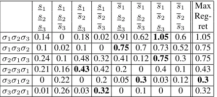
[.2, .8],s2 = [.3, .5]ands3 = [.1, .4]. For simplicity, assume that all operators have the same cost1and that the relation has cardinalityΩ = 1(so to get the real costs, the numbers in Table 1 just have to be multiplied by the true cardinality). To find the plan which minimises the maximum regret, we can perform an exhaustive enumeration of all possible execution plans under every possible scenario. We show later in Theorem 1 that it is sufficient to consider only the extreme scenarios since the worst case scenario for any plan is always an extreme one. Hence, if there arenoperators, we need to considern!different execution plans under each of2n

extreme scenarios. For our example, Table 1 shows the 48 regret values for the 6 possible plans under each of 8 extreme scenarios.

s₁ s₁ s₁ s₁ s1 s1 s1 s1 Max

s2 s2 s2 s2 s2 s2 s2 s2

Reg-s₃ s3 s3 s3 s3 s3 s3 s3 ret

σ1σ2σ3 0.14 0 0.18 0.02 0.91 0.62 1.05 0.6 1.05

σ1σ3σ2 0.1 0.02 0.1 0 0.75 0.7 0.73 0.52 0.75

σ2σ1σ3 0.24 0.1 0.48 0.32 0.41 0.12 0.75 0.3 0.75

σ2σ3σ1 0.21 0.16 0.43 0.42 0.2 0 0.4 0.1 0.43

σ3σ1σ2 0 0.22 0 0.2 0.05 0.3 0.03 0.12 0.3

σ3σ2σ1 0.01 0.26 0.03 0.32 0 0.1 0 0 0.32

Table 1: The regret for each plan under each scenario in Exam-ple 4.

Therefore, the optimal plan for scenariox1ispopt(x1)=σ3σ1σ2 and its cost is:

Cost(popt(x1), x1) = (1 +.1 +.1×.2) = 1.12 The regret of planp1under scenariox1using Equation (3) is:

γ(p1, x1) = Cost(p1, x1)−Cost(popt(x1), x1)

= 1.26−1.12 = 0.14

In order to find the minmax regret solution, the maximum regret of each plan needs to be found. For planp1, the maximum regret is

1.05which occurs in scenario(s1, s2, s3), its worst-case scenario. The maximum regret for each plan is shown in bold face in Table 1. Finally, we are looking for the plan with the smallest maximum regret (i.e., the smallest value in the last column of Table 1). As a result the minmax regret solution,M RO(S), is planσ3σ1σ2, which has the best performance among all plans when confronted with

their worst-case scenarios. 3

In the above example, it is interesting to consider which scenario gives rise to the maximum regret for each plan. Note that for each plan its worst-case scenario is one in which the operators in some initial sequence in the plan each take on their maximum selectiv-ity followed by the remaining operators taking on their minimum selectivity. We call such a scenario amax-minscenario.

DEFINITION 9. Letpbe the planσπ(1), σπ(2), . . . , σπ(n). A scenario forpis called amax-minscenario if there is a0≤k≤n

such that for all1≤i≤k,sπ(i)=sπ(i), and for allk+1≤i≤n,

sπ(i)=sπ(i).

So the firstkoperators inptake on their maximum selectivity, while the rest take on the minimum. Note that for a planpwithn

operators, there aren+1max-min scenarios. Max-min scenarios are the only scenarios considered by the max-min heuristic we develop in this paper. However, it is important to state that, in general, the worst-case scenario for a plan may not be a max-min scenario.

4.

PROPERTIES OF MRO

Before presenting algorithms for solving the MRO selection or-dering problem, we identify some of its important properties3.

In order to determine the worst-case scenario of a plan, i.e., the scenario for which a plan exhibits its largest regret, we only have to check extreme scenarios.

THEOREM 1. The worst-case scenario for any query planpis always an extreme scenario.

3

The proofs of results in this section and the next are published in a technical report available athttp://arxiv.org/abs/1507. 08257.

We can determine the relative order two operators have to be in to minimise the maximal regret if one operator dominates the other.

THEOREM 2. Ifσa dominatesσb, then there exists a planp

minimising the maximal regret in whichσaprecedesσb.

EXAMPLE 5. Recall from Example 4 the setS={σ1, σ2, σ3} of selection operators, with selectivitiess1= [.2, .8],s2= [.3, .5] ands3= [.1, .4]. Becauseσ3dominatesσ1andσ2, in the minmax regret solution, i.e. planσ3σ1σ2,σ3precedesσ1andσ2. As a result of domination, in this example we would only have to consider two plans when searching for the minmax regret solution. 3

For the TFT problem, Kasperski used the simple heuristic of sorting jobs in non-decreasing order according to the midpoints of their intervals, yielding a 2-approximation [17]. This approach does not guarantee a bound for MRO selection ordering; as shown below, the quality of the solution can become arbitrarily bad.

Given2n+ 1operators, the firstnoperators have the selectivities

si= 0andsi= 1(1≤i≤n), while the nextnoperators have the

selectivitiessi=si= 0.5 +(n+ 1≤i≤2n) for some small.

The final operator has a constant selectivity of1to guarantee that it will always be in last position, meaning that its selectivity will not impact any further steps.

The midpoint heuristic will order the operators in exactly this way, from 1 to2n+ 1. Clearly, the worst-case scenario for this plan is whensiis set to1for1≤si≤n. In the optimal plan for this

scenario, the operatorsσiwithn+ 1≤i≤2nwill be executed

first.

The regret of this plan is computed as follows:

1 + 12 . . . + 1n + f(n) − (0.5 +) − (0.5 +)2 _{. . . − (0.5 +)}n _{− g(n)}

wheref(n)andg(n)stand for the cost of the remaining operators in the plan. A lower bound for this expression is the following, since

f(n)≥g(n)(see Lemma 3 below):

n−n(0.5 +)

With increasingnand small values for, this expression can get arbitrarily large.

LEMMA 3. Given a query planpand a scenariox, we have the following relationship between the summands in Cost(p, x)and Cost(popt(x), x), wherepopt(x)is the optimal plan for scenariox:

k Y

j=1

sπ(j)≥

k Y

j=1

sπopt(x)(j)for allkwith1≤k≤n−1

In common with other MRO problems, we can show that the decision problem for generalM RO(S), which we callMINMAX REGRET, is NP-hard. In this version, we are given a setS =

{σ1, σ2, . . . , σn}of selection operators each having unit cost, as

well as a setX = {X1, X2, . . . , Xm}of scenarios, where each

scenarioXjspecifies a selectivitysijfor each operatorσi,1≤j≤

mand1≤i≤n.

MINMAX REGRET: given a setSofnselection operators, a setXof

mscenarios, and a real numberR, is there a plan whose maximum regret is less thanR?

We can show thatMINMAX REGRETis NP-hard by reducing a version ofSET COVERto it.

5.

SOME POLYNOMIAL-TIME CASES

In this section we show that, for sets of selection operatorsS

satisfying certain properties,M RO(S)can be found in polynomial time. In particular, we look at dominant operators, which can easily be ordered correctly, and their combination with constant operators, i.e., operators for which we can obtain exact selectivity values. As before, we assume that the cost of each operator is one.

LetSbe a set of selection operators such that the selectivity of each operator can be estimated accurately (i.e., each selectivity is constant). Then, as mentioned in Section 2.1,M RO(S)can be found by sorting the operators in non-decreasing order of their rank given by Equation (1). Given our assumption that each operator has cost one, findingM RO(S)reduces to sorting the operators in non-decreasing order of their selectivity alone.

Recall from Section 3.1 the definition of a dominant setS of operators. Given a dominant setSof operators, it follows from The-orem 2 that the minmax regret solution is one where the operators are sorted in non-decreasing order according to their minimum (or maximum) selectivity value. (Note that a set of constant operators is a special case of a dominant set of operators.) We therefore have:

COROLLARY 1. If S is a dominant set ofn operators, then

M RO(S)can be solved inO(nlogn)time.

When we include nested operators (recall the definition from Section 3.1), the problem becomes much more difficult. As a step in the direction of solving the general problem, we consider below the simple case of a strictly dominant set of operators (also defined in Section 3.1) along with a single constant operator nested within one of the non-constant operators. IfSis a strictly dominant set of operators, then the planM RO(S)has zero regret under all scenarios. This is because all operators inM RO(S)will be in the same position as in the corresponding optimal plan under all scenarios.

LetSbe a strictly dominant set which includes a constant operator

σcnested within one of the non-constant operators, sayσi. In this

case, we know how to place the dominant operators relative to each other inM RO(S)but we need to determine the position of

σcinM RO(S). Sincesi ≤ sc ≤ si, the constant operatorσc

should be either immediately before or immediately afterσi in

M RO(S). Interestingly, the correct position forσcdepends only

on the midpoint of the selectivitysiofσi.

PROPOSITION 1. LetSbe a strictly dominant set ofnoperators such thatM RO(S) = (σ1, . . . , σn). Letσcbe an operator with

constant selectivityscsuch thatsi≤sc≤si, for some1≤i≤n,

andS0=S∪ {sc}. InM RO(S0),σcis placed between (1)σi−1 andσiifsc≤(si+si)/2, or (2)σiandσi+1ifsc≥(si+si)/2.

Note that ifsc = (si+si)/2, thenσc can be placed either

betweenσi−1andσior betweenσiandσi+1inM RO(S0).

Proposition 1 can be generalised to the case in which each non-constant operator has at most one non-constant operator nested within it. An interesting observation about the situation described in Proposi-tion 1 is that the worst-case scenario is a max-min scenario.

PROPOSITION 2. LetSbe a strictly dominant set ofnoperators such thatM RO(S) = (σ1, . . . , σn). Letσcbe an operator with

constant selectivityscsuch thatsi≤sc≤si, for some1≤i≤n,

andS0 =S∪ {sc}. The scenario(s1, . . . , sj−1, sc, s_j, . . . , s_n),

in which eitherσj−1orσjis equal toσi, is a worst-case scenario

forM RO(S0).

6.

MAX-MIN HEURISTIC

Computing the regret of every selection ordering for every possi-ble scenario makes the brute-force algorithm infeasipossi-ble, since there aren!different orderings and2n_{scenarios, givennoperators. So in}

order to find an efficient heuristic, we have to significantly reduce the number of orderings and scenarios. While doing so, we want to leverage the insights gained from our theoretical investigation.

Let us first look at the number of possible scenarios. As we have seen in the previous section, max-min scenarios seem to play a special role when it comes to the maximum regret of a given plan

p. Intuitively this makes sense, as in an optimal plan many of the operatorsσilocated towards the beginning ofpwith selectivitiessi

will trade places with operatorsσjlocated towards the end ofpwith

selectivitiessj. Consequently, there tends to be a large difference

between the planpand an optimal plan for a max-min scenario, leading to a substantial (if not maximal) regret forp. So in our heuristic we aim to generate plans that perform well for max-min scenarios. This reduces the number of scenarios we have to consider from2n

ton+ 1.

We now turn to determining the order of the selection operators. There are two well-known basic methods for doing this (efficiently). The first one is constructing a plan by combining partial plans in a way that leads to an optimised execution order. Very often putting the partial plans together requires using a heuristic to solve a combinatorial problem. The second method is to quickly create a complete plan (e.g., by using a simple heuristic) and then try to improve the plan by rewriting it (e.g., by swapping or removing and re-inserting operators). In our approach we wanted to have both options available, so we decided to develop different variants. The complexity of our heuristic shows slight differences depending on the variant we use; however, the algorithms we apply all have polynomial complexity.

Our max-min heuristic algorithm,H(p, q), which is in fact a template for a number of algorithms, is shown as Algorithm 1. It is parameterised by two inputs:p, a (possibly empty) starting plan, andq, an order in which to process operators. Clearly, to generate a complete plan the union ofpandqhas to contain all the operators. If the intersection ofpandqis empty, our algorithm is similar to insertion sort: in turn, we consider each operator inqand place it intopat the position that minimises the regret over all max-min scenarios. If an operator inqis already present inp, then we remove it frompbefore re-inserting it. This is equivalent to moving an operator to a different position. Again we determine the position minimising the regret over all max-min scenarios.

Algorithm 1:H(p, q)

1 foreachoperatortfrom the sequenceqdo

2 iftis inpthenremovetfrompAssumepcurrently

comprisesioperators;

3 foreachpositionj,1≤j≤i+ 1, inpdo

4 Temporarily inserttin positionjinp; 5 foreachmax-min scenario forpdo 6 Calculate the regret of planp;

7 Store the maximum regret for positionj;

8 Choose as the final position fortinpthat which minimises

the maximum regret;

9 Returnp;

con-sideri+ 2max-min scenarios. Calculating the regret of a plan with

noperators can be done in timeO(nlogn). Hence the algorithm described above has an overall complexity ofO(n4logn)(in the worst casei=nfor every execution of the outer loop). However, by computing costs incrementally when an operator moves position and one max-min scenario moves to the next, we can implement the heuristic to run in timeO(n3₎

.

EXAMPLE 6. Recall from Example 5 the setS={σ1, σ2, σ3} of selection operators, with selectivitiess1= [.2, .8],s2= [.3, .5] ands3 = [.1, .4]. Consider our max-min heuristic algorithm,

H(p, q), with initial planp=σ3σ1and remaining operatorq=σ2. Sincepconsists of two operators,σ2should be checked in three positions: beforeσ3, afterσ1and between them. For each posi-tion and resulting plan, the regret is calculated under all max-min scenarios, of which there are four in this example.

As an example, consider the plan in whichσ2 is placed be-tweenσ3andσ1. The regret will be calculated for the scenarios

(s₃, s₂, s₁), (s3, s2, s1), (s3, s2, s1)and(s3, s2, s1). The maxi-mum regret for this plan is0.3which occurs in scenario(s3, s2, s1). Finally, the solution will be the plan with the smallest maximum regret, which happens to beσ3σ2σ1. As a matter of fact, the solution returned by the max-min heuristic is the same as the actual minmax regret solution, as was shown in Example 4. 3

In the following two subsections, we consider various criteria for choosing an initial plan and for ordering the remaining operators.

6.1

Choosing an Initial Plan

Even though we can run our heuristic with an empty initial planp, i.e., building a solution by inserting all operators one by one, often it makes sense to start with a prebuilt partial plan.

One particular and important case is that of dominant operators. Given a setSof operators, if we can identify a subsetS0 ⊆Sof dominant operators, we know that we can find an optimal solution

p0forS0quickly and that the relative order of the operators inp0

will not change in any optimal plan forS(see Theorem 2). Thus, takingp0as the initial plan when callingH(p, q)makes good sense. However, there may be different ways to chooseS0, as in general there may be more than one such dominant set. If we have more than one option, we can use the following criteria to make a deci-sion: choose the subsetS0(1) with the maximum cardinality or (2) whose operators have the largest total width. While the intuition in choosing the largest subset is clear, the motivation for maximising the width may not be so evident: the wider an interval, the more impact it has on the solution, so it is more important to slot wide intervals into the correct positions. As we often encountered several subsets sharing the same maximum cardinality, we introduced a tie-breaker: choose the subsetS0(3) with the maximum cardinality whose total width is greatest. In our experiments, we found that this third approach gave the best overall results.

EXAMPLE 7. Recall from Example 6 the setS={σ1, σ2, σ3} of selection operators, with selectivitiess1= [.2, .8],s2= [.3, .5] ands3= [.1, .4]. SetShas two dominant subsets:S1 ={σ1, σ3} andS2 = {σ2, σ3}. Both obviously satisfy criterion (1) above, being of maximum cardinality. However, if we use criterion (2), namely the set which has operators with the largest total selectivity width, then we will chooseS1since its total width is0.9while that ofS2is0.5.S1would also be chosen according to criterion (3).

After choosing the preferable subset, we need to produce initial planpby sorting the operators in nondecreasing order of their minimum (or maximum) selectivities. Therefore,p=σ3σ1whenS1 is chosen, whilep=σ3σ2ifS2is chosen. 3

Having an initial plan allows us to combine our algorithm with other heuristics. We can take the output of another algorithm as our initial planpand then refine this result by runningH(p, q)on it. Moreover, we can use the output ofH(p, q)as input for another iteration of our own heuristic.

6.2

Ordering Criteria

Since our algorithm makes only a single pass over all the operators when (re-)inserting them into the plan, the order in which operators are considered may have a significant impact on the final outcome. For example, when inserting selections into an empty initial plan, operators considered earlier are tested in fewer positions relative to each other compared to those considered later.

We have considered two different ordering criteria in our ex-periments: intervalmidpoint(denoted byM) and intervalwidth

(denoted byW). Given a selectivity intervals = [s, s], the mid-point ofsis(s+s)/2while the width ofsis s−s. In each case, operators can be ordered by non-decreasing (denoted+) or non-increasing (denoted−) values. Overall, the ordering criteria are denoted byM+,M−,W+andW−. So, for example,W+

stands for operators being considered in non-decreasing order of their selectivity interval width.

7.

EXPERIMENTAL RESULTS

We evaluated the max-min heuristic experimentally, measuring the impact of different parameters on its performance. We also implemented the brute-force algorithm for finding optimal solutions in order to evaluate how well the heuristic performs.

A commodity PC, with 8 GB RAM, Intel Core i5 processor running at 3.19 GHz and Windows 7 Enterprise (64-bit), was used to perform the experiments. The minmax regret brute-force algorithm and max-min heuristic were implemented in Java and compiled with the Eclipse IDE (Juno release), which is JDK compliant and uses the JavaSE-1.7 execution environment. The Star Schema Benchmark (SSB) queries were run on a simulation platform written in Ruby 1.9.3.

7.1

Generating Test Data

We first generated a synthetic data set to investigate the perfor-mance of our heuristic. Each test case corresponded to a set ofk

selection operators, withkranging from 2 to 10, and for eachkwe generated a hundred different sets. Whilek= 2is not hard to solve, it was included for verification purposes (any heuristic has to be able to find the optimal plan for this simple case). Ten operators was the upper limit we were able to solve optimally, checking10!·210

(≈3.7 billion) different costs for each test case. For each set of selection operators we determined the lower and upper bounds of their selectivity intervals by generating2kuniformly distributed random numbers between 0 and 1.

For real-world data, we used the Enron email data set, as intro-duced in Example 1. Once again, test queries used from 2 to 10 operators/predicates. For eachn∈[2,10], 20 queries were gener-ated, each with one predicate onsubjectandn−1predicates on

body. The 20 queries were generated by randomly selecting from 40 keywords forsubjectand 45 keywords forbody, and were checked to ensure that each returned a nonempty answer.

a conjunctive predicate whose clauses are made up of the selected attributes compared to a random value taken from the attribute’s domain, using a less-than or greater-than operator. The following predicate is an example generated in our experiments:

orderKey < 2964443 and linenumber > 5 and quantity < 29.

7.2

Parameters

For the synthetic and Enron data sets, we looked at the effects of the ordering criteria and the choice of initial plan on the quality of our heuristic. Additionally, we investigated the impact of running our heuristic multiple times, using the output of one phase as the initial plan of the next phase.

We measure the performance of our heuristic by defining the

regret ratioλ(S), which is the regret computed byH(p, q)divided by the optimal regret. More formally, given a setS of selection operators, let us denote the set of possible plans byP(S)and the set of possible scenarios byX(S). Recall from Section 3.1 that

R(P(S), X(S))then denotes the optimal regret. Then

λ(S) =R(H(p, q), X(S))

R(P(S), X(S))

We only calculateλ(S)using the above formula when the optimal minmax regret is non-zero. As mentioned in Section 5, the optimal minmax regret is zero only whenS forms a strictly dominating set. For such cases, our max-min heuristic always finds the optimal minmax regret solution, so we defineλ(S)to be one.

In view of having multiple test cases per number of selection operators, we calculate theaverage regret ratioand theworst regret ratio(simply the maximum value ofλ(S)).

For the Enron data, we calculated selectivity intervals for the

likepredicates as described in the Introduction. For each selected keyword, we ran queries to find the minimum selectivity (given by exact matches of the keyword) and the maximum selectivity (given by the minimum selectivity of all 2-grams of the keyword). This gave rise to a range of intervals: those with small values such as

[0.0004,0.01]for keyword ‘progress’ in thesubject, those with larger values such as[0.6,0.7]for ‘you’ in thebody, and those with a big range such as[0.07,0.6]for ‘price’ in thebody.

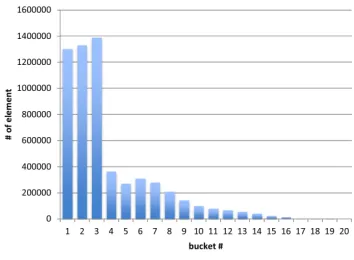
For the Star Schema Benchmark we created some very rudi-mentary histograms by dividing the domain of an attribute into equal-sized ranges, counting the number of tuples that fall into each range. We do not keep any further information on the distribution of tuples within each range of a histogram. For example, Figure 1 shows the histogram for the attribute ordtotalprice, consisting of 20 ranges each covering roughly 18,000 different values, e.g., bucket #1 covers the range from 1 to 17,673.

Figure 1: Histogram for attribute ordtotalprice.

This basic information allows us to determine intervals for the selectivities of selection operators. For a “less than” / “greater than” operator, we know that all histogram ranges exclusively covering smaller/larger values have to be included fully. However, for the range the predicate value falls into, we do not know precisely how many elements will be selected. In extreme cases, none or all of the elements satisfy the predicate, giving us the lower and upper bound for the selectivity. Example 8 illustrates this with concrete values.

EXAMPLE 8. Given the histogram for attributeXbelow and the predicateX <126, we can compute the lower bound and upper bound for the selectivity as follows: lower bound = 200

1000 = 0.2,

upper bound =200+100₁₀₀₀ = 0.3. 3

Range # of elements 1-100 200 101-200 100 201-300 400 301-400 300

Many sophisticated query optimisation techniques, such as least expected cost (LEC), assume that they have access to probability dis-tributions of parameter values. LEC needs this to be able to compute utilities [7]. However, in our case we only have very rudimentary statistics, since we do not know anything about the distribution of attribute values within a range. The best we can do is to fall back on the assumption of uniform distribution, approximating the distribu-tion using a mean value (this is also what least specific cost (LSC) optimisation would do in this case). For example, applying this method to the numbers given in Example 8 would yield a selectivity of 0.225 for the predicateX < 126. We compare our minmax regret optimisation technique to a mean-value-based approach using SSB data. Additionally, we do a comparison with a simple midpoint heuristic, i.e., sorting the intervals in non-decreasing order of their midpoint.

7.3

Results

First we present the results obtained studying the different variants of the max-min heuristic on the synthetic and Enron data, and then move on to the Star Schema Benchmark results.

7.3.1

Synthetic and Enron Data Sets

We experimented with a number of operator ordering criteria and initial plans for the max-min heuristic. These included starting with an empty initial plan (∅), considering random operator ordering (U), ordering by midpoint (M- and M+) and ordering by width (W- and W+). We briefly summarise the findings of our experiments here. Overall, the W+ ordering (non-decreasing width) performed best with an overall average regret ratio of 1.03 and an overall worst regret ratio of 1.94. W- was often even worse than a random order, while M+ and M- sometimes generated plans whose regret ratio was above 3. We also ran a midpoint heuristic that simply ordered the intervals in non-decreasing order of their midpoints (not going through all max-min scenarios). The midpoint heuristic was often worse than running the max-min heuristic with a random order.

2 4 6 8 10 0

0.2 0.4 0.6 0.8 1

total number of operators

%

of

cases

with

exact

solution

midpoint (∅,U) (D:CW,W+) ((D:CW,W+),W+) (((D:CW,W+),W+),W+)

2 4 6 8 10

1 2 3 4

total number of operators

w

orst

re

gret

ratio

midpoint (∅,U) (D:CW,W+) ((D:CW,W+),W+) (((D:CW,W+),W+),W+)

2 4 6 8 10

1 1.05 1.1 1.15 1.2

total number of operators

av

erage

re

gret

ratio midpoint_(∅,U)

(D:CW,W+) ((D:CW,W+),W+) (((D:CW,W+),W+),W+)

(a) Percentage of exact solutions (b) Worst regret ratio (c) Average regret ratio

Figure 2: Results for synthetic data set.

2 4 6 8 10

0 0.2 0.4 0.6 0.8 1

total number of operators

%

of

cases

with

exact

solution

midpoint (∅,U) (D:CW,W+) ((D:CW,W+),W+) (((D:CW,W+),W+),W+)

2 4 6 8 10

1 1.5 2 2.5 3

total number of operators

w

orst

re

gret

ratio

midpoint (∅,U) (D:CW,W+) ((D:CW,W+),W+) (((D:CW,W+),W+),W+)

2 4 6 8 10

1 1.05 1.1 1.15 1.2

total number of operators

av

erage

re

gret

ratio midpoint₍∅,U) (D:CW,W+) ((D:CW,W+),W+) (((D:CW,W+),W+),W+)

(a) Percentage of exact solutions (b) Worst regret ratio (c) Average regret ratio

Figure 3: Results for Enron data set.

results for the worst case regret ratio were rather inconclusive, so we tried to improve on this by running multiple phases of our heuristic. Figures 2(a), (b) and (c) show the results for running our heuristic multiple times. This means that we take the output of running one phase of our heuristic and use it as the initial plan for the next phase. The figures show the results for starting off by running (D:CW, W+) first and then executing two more phases.

As can be seen, this variant clearly outperforms the baseline algorithm (∅,U), the midpoint heuristic, and the other variants in all respects. For example, for 10 operators, the worst regret ratio is less than1.23and the average ratio is approximately1.01, compared to approximately1.94and1.08, respectively, for running only a single phase of the heuristic. Moreover, running one additional phase improves the quality of the generated plan significantly, but running another phase makes almost no difference.

The results on the Enron data set (Figure 3) showed similar trends, but were more impressive in every respect. The two- and three-phase variants of the max-min heuristic found the minmax optimal solution in 84% of cases, had a worst regret ratio of only 1.05, and an average regret ratio of less than 1.001. By contrast, the midpoint heuristic had a worst regret ratio of over 1.49, an average of 1.06, and did not find single minmax optimal solution with 10 operators.

To highlight how bad a poor choice of selectivity can be, we also tested using the minimum selectivity values of the intervals (as would be done if estimates were based simply on the selectivity of the keywords themselves). This produced a worst case regret ratio ofalmost 30 for only 5 operators.

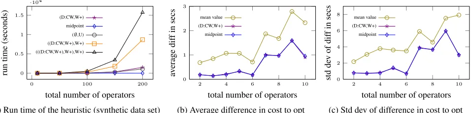
Figure 4(a) shows the run time of the W+ ordering variant (sin-gle and multiple phases) together with the baseline algorithm (∅,U) when generating plans for up to 200 operators using the synthetic data set (the run times on the Enron data set were similar). Unsur-prisingly, the variants midpoint, (∅,U), and (D:CW,W+) have the fastest run times, as they only sort a set of operators or execute a single operator insertion phase. Furthermore, it can be clearly seen

that the additional run time of (((D:CW,W+),W+),W+) does not pay off, since it produces plans that are only marginally better than those of ((D:CW,W+),W+).

7.3.2

Star Schema Benchmark

We optimised the generated SSB queries using minmax regret optimisation, a mean-value-based approach, and also computed the optimal execution plan using exact selectivities, which means that we are comparing actual query plan costs rather than regret ratios.

Figure 4(b) shows the results for the average difference in costs between the query execution plans generated by different methods and the optimal plan (every data point in the diagram averages the measurement obtained by running 100 different queries). We only include two variants of minmax regret optimisation, (D:CW,W+) and the simple midpoint heuristic, as for SSB no major differences were discernible between the different variants in terms of the quality of the query plans. Surprisingly, the midpoint heuristic, although not very good at optimising the regret ratio, seems to produce efficient query execution plans. Considering the fact that all queries had an average run time between 60 and 80 seconds, the numbers shown in Figure 4(b) may not seem like a big difference. However, this shows that minmax regret optimisation delivers better plans than a mean-value-based approach.

0 100 200 0

0.5 1 1.5

·104

total number of operators

run

time

(seconds)

(D:CW,W+) midpoint (∅,U) ((D:CW,W+),W+) (((D:CW,W+),W+),W+)

2 4 6 8 10

0 1 2 3

total number of operators

av

erage

dif

f

in

secs mean value

(D:CW,W+) midpoint

2 4 6 8 10

0 2 4 6 8

total number of operators

std

de

v

of

dif

f

in

secs mean value (D:CW,W+) midpoint

(a) Run time of the heuristic (synthetic data set) (b) Average difference in cost to opt (c) Std dev of difference in cost to opt

Figure 4: Results on run time (synthetic data set) and difference in cost to optimal (SSB).

8.

CONCLUSION

We have investigated query optimisation under partial ignorance, in particular ordering selection operators optimally if their selec-tivities are defined by an interval rather than an exact value. The strategy we employed, minmax regret optimisation (MRO), is con-sidered to be a pessimistic approach compared to other techniques from decision theory. In our opinion this makes it well-suited to query optimisation in database systems, which should be about avoiding bad plans rather than finding the best one. There is one major drawback, though: selection ordering under MRO becomes NP-hard. However, we have shown that special cases can be solved efficiently and that heuristics can quickly find good solutions.

For future work we plan to extend our approach to costs described by intervals and relative regret, i.e., considering the ratio of the cost of a plan to the optimal plan for a scenario rather than the difference. Also interesting are other operators, such as joins, whose ordering is heavily influenced by selectivities as well and suffers from similar issues: it is hard to obtain exact values. Further topics we would like to tackle are finding approximation algorithms with proven bounds and modelling correlation of query predicates. Nevertheless, we think this is an important first step in discovering new approaches for making query optimisers more robust and one of our medium term goals is to build a general framework for query optimisation under partial ignorance.

9.

REFERENCES

[1] H. Aissi et al. Min-max and min-max regret versions of combinatorial optimization problems: A survey.European J. of Operational Research, 197(2):427–438, 2009.

[2] R. Avnur and J. M. Hellerstein. Eddies: continuously adaptive query processing. InSIGMOD, pages 261–272, 2000. [3] B. Babcock and S. Chaudhuri. Towards a robust query

optimizer: a principled and practical approach. InSIGMOD, pages 119–130, 2005.

[4] S. Babu, P. Bizarro, and D. DeWitt. Proactive re-optimization. InSIGMOD, pages 107–118, 2005.

[5] S. Babu et al. Adaptive ordering of pipelined stream filters. In

SIGMOD, pages 407–418, 2004.

[6] S. Chaudhuri et al. Selectivity estimation for string predicates: Overcoming the underestimation problem. InICDE, pages 227–238, 2004.

[7] F. Chu et al. Least expected cost query optimization: an exercise in utility. InPODS, pages 138–147, 1999.

[8] F. Chu et al. Least expected cost query optimization: what can we expect? InPODS, pages 293–302, 2002.

[9] H. D, P. N. Darera, and J. R. Haritsa. On the production of anorexic plan diagrams. InVLDB, pages 1081–1092, 2007. [10] A. Deshpande et al. Exploiting correlated attributes in

acquisitional query processing. InICDE, pages 143–154, 2005.

[11] S. Ganguly. Design and analysis of parametric query optimization algorithms. InVLDB, pages 228–238, 1998. [12] M. Garofalakis and P. B. Gibbons. Wavelet synopses with

error guarantees. InSIGMOD, pages 476–487, 2002. [13] J. M. Hellerstein and M. Stonebraker. Predicate migration:

optimizing queries with expensive predicates. InSIGMOD, pages 267–276, 1993.

[14] Y. Ioannidis. The history of histograms (abridged). InVLDB, pages 19–30, 2003.

[15] S. M. Johnson. Optimal sequential testing. RAND Research Memorandum RM1652, RAND Corporation, 1956. [16] N. Kabra and D. J. DeWitt. Efficient mid-query

re-optimization of sub-optimal query execution plans. In

SIGMOD, pages 106–117, 1998.

[17] A. Kasperski.Discrete Optimization with Interval Data -Minmax Regret and Fuzzy Approach. Springer, 2008. [18] R. Krishnamurthy, H. Boral, and C. Zaniolo. Optimization of

nonrecursive queries. InVLDB, pages 128–137, 1986. [19] V. Lebedev and I. Averbakh. Complexity of minimizing the

total flow time with interval data and minmax regret criterion.

Discrete Appl. Math., 154(15):2167–2177, Oct. 2006. [20] G. Lohman. Is query optimization a “solved” problem?

http://wp.sigmod.org/?p=1075, 2014.

[21] V. Markl et al. Robust query processing through progressive optimization. InSIGMOD, pages 659–670, 2004.

[22] V. Markl et al. Consistent selectivity estimation via maximum entropy.The VLDB Journal, 16(1):55–76, Jan. 2007. [23] G. Moerkotte et al. Exploiting ordered dictionaries to

efficiently construct histograms with q-error guarantees in SAP HANA. InSIGMOD, pages 361–372, 2014.

[24] T. Neumann and C. A. Galindo-Legaria. Taking the edge off cardinality estimation errors using incremental execution. In

BTW, pages 73–92, 2013.

[25] M. Peterson.An Introduction to Decision Theory. Cambridge University Press, 2009.

[26] N. Polyzotis and M. Garofalakis. Statistical synopses for graph-structured XML databases. InSIGMOD, pages 358–369, 2002.

[27] T. Rabl et al. Variations of the star schema benchmark to test the effects of data skew on query performance. InICPE, pages 361–372, 2013.

[28] U. Srivastava et al. Operator placement for in-network stream query processing. InPODS, pages 250–258, 2005.

[29] V. Zadorozhny et al. Efficient evaluation of queries in a mediator for websources. InSIGMOD, pages 85–96, 2002. [30] N. Zhang et al. Statistical learning techniques for costing