Using Different Machine Learning Techniques for Predicting the Price of
Used Cars
Harikrushna Vanpariya
M.Tech
Department of Computer Science & Technology
Abstract— In this paper, various machine learning techniques investigates to predict used car price in India. The prediction is based on the historical data and the data is fetched from various website which is selling the used cars. Here the predictions are made with different techniques like, M5P, Random Tree, Random Forest, K nearest neighbors, K*, Fast decision tree and various regression methods. We have derived the top prediction methods post analyzing above prediction methods.
Key words: Machine Learning, Regression, Used Cars, Prediction
I. INTRODUCTION
With increasing numbers of vehicles, resale of the vehicle is also increased, so to identify the correct resale price is also important while selling a vehicle. India had 55,725,543 four wheelers by 2015 [1]. With such a high number of vehicales in the country, it is really interesting problem to solve the resale price of a vehicle.
Predicting the resale value of a car is not a simple task. The value of used cars depends on a number of factors. The most important ones are usually the age of the car, its make (and model), the origin of the car (the original country of the manufacturer), its mileage (the number of kilometers it has run) and its horsepower. Due to rising fuel prices, fuel economy is also of prime importance. Unfortunately, in practice, most people do not know exactly how much fuel their car consumes for each km driven. Other factors such as the type of fuel it uses, the interior style, the braking system, acceleration, the volume of its cylinders (measured in cc), safety index, its size, number of doors, paint colour, weight of the car, consumer reviews, prestigious awards won by the car manufacturer, its physical state, whether it is a sports car, whether it has cruise control, whether it is automatic or manual transmission, whether it belonged to an individual or a company and other options such as air conditioner, sound system, power steering, cosmic wheels, GPS navigator all may influence the price as well. The look and feel of the car certainly contributes a lot to the price. As we can see, the price depends on a large number of factors. Unfortunately, information about all these factors are not always available and the buyer must make the decision to purchase at a certain price based on few factors only. [2]
In this paper, we are covering very small set of data and a specific model of the car which is widely used by customer in India.
In section III we analyze the different Machine Learning techniques and in section IV, we will provide overall comparison for the data we are using.
Weka [15] is used to analyse the different techniques of Machine Learning.
II. INPUT DATA DETAILS
The data is collected from the various websites [3] which are selling the used car. The below data was collected for each car. It contains, Year of made, Model of Car, Engine Liter (1Liter = 1000 cc), Engine Type (Automatic or manual engine), Kilometers driven and the resale price.
In India, the capacity of engine is measured based on the Liters. Engine displacement is the swept volume of all the pistons inside the cylinders of a reciprocating engine in a single movement from top dead center (TDC) to bottom dead center (BDC). It is commonly specified in cubic centimetres (cc or cm3) [4]. We have collected 2000+ used car’s data from the website, which we later prun and provided the analysis for only Hyundai i10 all varients.
Year Model
Engine Liter (1L=1000
cc)
Engine Type
Kms Driver
Price INR (in
Lacs)
2016 Asta 1.2 AT 7822 6.22
2016 Asta 1.2 AT 7822 6.22
2016 Sportz 1.2 MT 22172 5.24
2016 Sportz 1.2 MT 22172 5.24
2016 Sportz 1.2 MT 34518 5.04
2016 Sportz 1.2 MT 34518 5.04
2014 Sportz 1.2 MT 34757 4.9
2014 Sportz 1.2 MT 34757 4.9
2015 Asta 1.1 MT 47408 5.36
2015 Asta 1.1 MT 47408 5.36
2014 Sportz 1.2 MT 29342 4.87
2016 Asta 1.2 MT 5576 6.25
2016 Asta 1.2 MT 5576 6.25
2015 Magna 1.2 MT 21513 5.15
2015 Magna 1.2 MT 21513 5.15
2015 Asta 1.2 MT 12411 4.8
2015 Asta 1.2 MT 12411 4.8
2017 Sportz 1.2 AT 14611 6.75
2017 Sportz 1.2 AT 14611 6.75
2014 Asta 1.2 MT 21360 5.1
2014 Asta 1.2 MT 21360 5.1
2015 Asta 1.2 AT 7832 6.75
2015 Asta 1.2 AT 7832 6.75
2016 Sportz 1.2 MT 7575 5.5
2016 Sportz 1.2 MT 7575 5.5
Table 1: Sample Data for Hyundai I10 Grand
III. MACHINE LEARNING TECHNIQUES
A. M5P
Weka's M5P algorithm is a coherent modernization with several developments of the original M5 algorithm invented by R. Quinlan. This procedure offered the advantages of knowledge discovery through analyzing the patterns in the Bucharest Stock Exchange average daily trading. It incorporated a large amount of statistics, learns efficiently and automatically produced multirule combinations over a set of data and also applies a more computationally efficient strategy to build linear models, as it follows [7]:
Primary built a piecewise constant tree;
Followed by a linear regression model to the data in each leaf node.
The approach used in the M5 trees was to reduce the intrasubset deviation in the resulted values behind each branch [6], the splitting process being completed when the output values of all the instances that reach the node varied only vaguely, and only a small number of instances were left. [8].
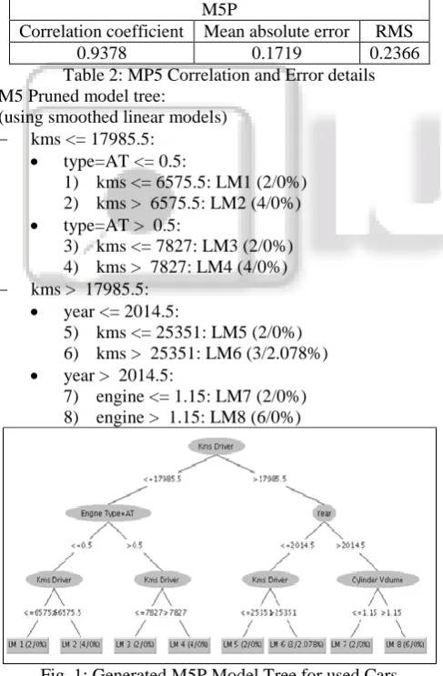
Here it generates the model tree with Correlation coefficient, mean absolute error and root mean squared error with the M5P for the input data set.
M5P
Correlation coefficient Mean absolute error RMS
0.9378 0.1719 0.2366
Table 2: MP5 Correlation and Error details M5 Pruned model tree:
(using smoothed linear models) kms <= 17985.5:
type=AT <= 0.5:
1) kms <= 6575.5: LM1 (2/0%) 2) kms > 6575.5: LM2 (4/0%) type=AT > 0.5:
3) kms <= 7827: LM3 (2/0%) 4) kms > 7827: LM4 (4/0%) kms > 17985.5:
year <= 2014.5:
5) kms <= 25351: LM5 (2/0%) 6) kms > 25351: LM6 (3/2.078%) year > 2014.5:
[image:2.595.46.290.323.695.2]7) engine <= 1.15: LM7 (2/0%) 8) engine > 1.15: LM8 (6/0%)
Fig. 1: Generated M5P Model Tree for used Cars
B. RandomTree
Random Tree is a supervised Classifier; it is an ensemble learning algorithm that generates many individual learners. It employs a bagging idea to produce a random set of data for constructing a decision tree. In standard tree each node is split
using the best split among all variables. In a random forest, each node is split using the best among the subset of predicators randomly chosen at that node.
Random trees have been introduced by Leo Breiman and Adele Cutler. The algorithm can deal with both classification and regression problems. Random trees is a collection (ensemble) of tree predictors that is called forest. The classification works as follows: the random trees classifier takes the input feature vector, classifies it with every tree in the forest, and outputs the class label that received the majority of “votes”. In case of a regression, the classifier response is the average of the responses over all the trees in the forest.
Random Trees are essentially the combination of two existing algorithms in Machine Learning: single model trees are combined with Random Forest ideas. Model trees are decision trees where every single leaf holds a linear model which is optimised for the local subspace described by this leaf. Random Forests have shown to improve the performance of single decision trees considerably: tree diversity is generated by two ways of randomization. First the training data is sampled with replacement for each single tree like in Bagging. Secondly, when growing a tree, instead of always computing the best possible split for each node only a random subset of all attributes is considered at every node, and the best split for that subset is computed. Such trees have been for classification Random model trees for the first time combine model trees and random forests. Random trees employ this produce for split selection and thus induce reasonably balanced trees where one global setting for the ridge value works across all leaves, thus simplifying the optimization procedure. [9] [10] [11] [12]
Following are the analysis for the Random Tree for the used car price.
Random Tree
Correlation coefficient Mean absolute error RMS
0.9925 0.0394 0.0931
Table 3: Random Tree Correlation and Error details Random Tree used for the prediction:
type = AT
| kms < 7827: 6.22 (2/0) | kms >= 7827: 6.75 (4/0) type = MT
| kms < 6575.5: 6.25 (2/0) | kms >= 6575.5
| | engine < 1.15: 5.36 (2/0) | | engine >= 1.15
| | | year < 2015.5 | | | | varient = Asta
| | | | | kms < 16885.5: 4.8 (2/0) | | | | | kms >= 16885.5: 5.1 (2/0) | | | | varient = Sportz: 4.89 (3/0) | | | | varient = Magna: 5.15 (2/0) | | | year >= 2015.5
| | | | kms < 14873.5: 5.5 (2/0) | | | | kms >= 14873.5
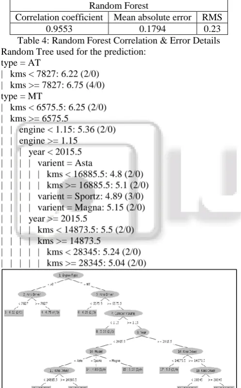
Fig. 1: Generated Random Tree for used car price Following are the analysis for the Random Forest for the used car price.
Random Forest
Correlation coefficient Mean absolute error RMS
0.9553 0.1794 0.23
Table 4: Random Forest Correlation & Error Details Random Tree used for the prediction:
[image:3.595.44.293.233.634.2]type = AT
| kms < 7827: 6.22 (2/0) | kms >= 7827: 6.75 (4/0) type = MT
| kms < 6575.5: 6.25 (2/0) | kms >= 6575.5
| | engine < 1.15: 5.36 (2/0) | | engine >= 1.15
| | | year < 2015.5 | | | | varient = Asta
| | | | | kms < 16885.5: 4.8 (2/0) | | | | | kms >= 16885.5: 5.1 (2/0) | | | | varient = Sportz: 4.89 (3/0) | | | | varient = Magna: 5.15 (2/0) | | | year >= 2015.5
| | | | kms < 14873.5: 5.5 (2/0) | | | | kms >= 14873.5
| | | | | kms < 28345: 5.24 (2/0) | | | | | kms >= 28345: 5.04 (2/0)
Fig. 2: Generated Random Forest model for used car price
C. Linear Regression Model
Linear regression is the most basic and frequently used predictive model for analysis. Regression estimates are generally used to describe the data and elucidate relationship between one or more independent and dependent variables. Linear regression finds the best-fit through the points, graphically. The best-fit line through the points is known as the regression line.
(1) is the price estimation equation for used car based on the sample data.
Estimation equation for Linear Regression: price = (0.15 * year) + (-7.2279 * engine) + (1.0062 * type=AT) +
(-0 * kms) + -287.9176
(1)
Linear Regression
Correlation coefficient Mean absolute error RMS
0.8967 0.2304 0.3277
Table 5: Linear Regression Correlation and Error details
D. K Nearest Neighbour Classifier
KNN (IBk in Weka) [15] are instance-based or lazy learners. It delays the process of modeling the training data until it is needed to classify the test samples. It can be used both for classification and prediction.
The training samples are described by n-dimensional numeric attributes. The training samples are stored in an n-dimensional space. When a test sample (unknown class label) is given, the k-nearest neighbor classifier searches the k tranining samples which are clsoest to the unknown sample. Closeness is usually defined in terms of Eucliedean distance.
With use of Weka we have created prediction model with KNN with instnace based classification. As Table VI. Depicts KNN has very high correlation coefficient which means it could able to classifies the majority of the cars with the correct price.
K nearst neighbour
Correlation coefficient Mean absolute error RMS
0.9969 0.0172 0.0569
Table 6: K Nearest Neighbour Correlation and Error details
E. K* Classifier
K-star or K* is an instance-based classifier. The class of a test instance is based on the training instances similar to it, as determined by some similarity function. It differs from other instance-based learners in that it uses an entropy-based distance function. Instance-based learners classify an instance by comparing it to a database of pre-classified examples. The fundamental assumption is that similar instances will have similar classifications. The question lies in how to define “similar instance” and “similar classification”. The corresponding components of an instance-based learner are the distance function which determines how similar two instances are, and the classification function which specifies how instance similarities yield a final classification for the new instance [14].
We used K* algorithm to derive the price of used car with the same data set and we observed that is has the same correlation coeffiecient as K nearest neighbour.
K* Algorithm
Correlation coefficient Mean absolute error RMS
0.9969 0.0172 0.0569
Table 7: K* Correlation and Error details
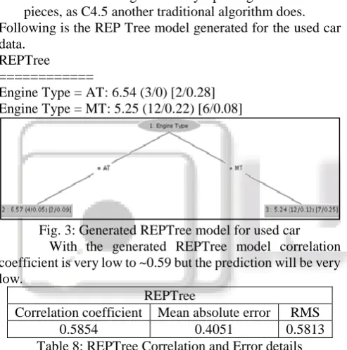
F. REPTree classifier
REPTree generates regression trees [5] based on information gain as the splitting principle, using reduces-error pruning, and sorts values for numeric attributes once.
The REPtree method built a regression tree using information gain/variance reduction and pruned it using reduced-error pruning in the following manner [9]:
Only sorted values for numeric attributes once due to its speed optimization;
Dealt with missing values by splitting instances into pieces, as C4.5 another traditional algorithm does. Following is the REP Tree model generated for the used car data.
REPTree ============
[image:4.595.311.546.98.238.2]Engine Type = AT: 6.54 (3/0) [2/0.28] Engine Type = MT: 5.25 (12/0.22) [6/0.08]
Fig. 3: Generated REPTree model for used car With the generated REPTree model correlation coefficient is very low to ~0.59 but the prediction will be very low.
REPTree
Correlation coefficient Mean absolute error RMS
0.5854 0.4051 0.5813
Table 8: REPTree Correlation and Error details
G. Additive Regression
Additive Regression enhances the performance of a regression base classifier. Each iteration fits a model to the residuals left by the classifier on the previous iteration. Prediction is accomplished by adding the predictions of each classifier. Reducing the shrinkage (learning rate) parameter helps prevent overfitting and has a smoothing effect but increases the learning time
With the use of Additive regression, we could achive the Correlation coefficient as 0.95. Equation (2) is the predictive classification of the additive regression.
Additive Regression
Correlation coefficient Mean absolute error RMS
0.9535 0.1654 0.2055
Table 9: Additive Regression Correlation and Error details Kms Driver <= 10121.5: 0.0592255243732158 Kms Driver > 10121.5: -0.03158694633238176 Kms Driver
is missing: 6.033820786006285E-19
(2)
IV. COMPARE RESULTS
We try to put all the results and identify the best technique to predict the used car value.
Overall Results
Machine Learning Method Correlation coefficient
M5P 0.9378
Random Tree 0.9925
Random Forest 0.9553
Linear Regression 0.8967
K nearst neighbour 0.9969
K* ( K-star ) 0.9969
REPTree 0.5854
[image:4.595.46.293.273.522.2]Additive Regression 0.9535
Table 10: Comparison of different ML Techniques In Table X. we can see K nearest neighbour and K* is the best prediction technique for identifying the used car.
V. CONCLUSION
This work examines the different Machine Learning technique for predicting the price of the used car. We could able to conclude that the K nearest neighbour or K* algorithm is the best fit for predicting price of a used car.
Currently this analysis is performed for only one brand of car which can be extended to multiple brands and also with few additional parameters like the damage to the car and state.
REFERENCES
[1] https://en.wikipedia.org/wiki/List_of_countries_by_veh icles_per_capita#cite_note-30
[2] Predicting the Price of Used Cars using Machine Learning Techniques. 2014. , International Journal of Information & Computation Technology., ISSN 0974-2239 Volume 4, Number 7 (2014), pp. 753-764 [3] http://www.truebil.com/used-cars-in-bangalore/ [4] https://en.wikipedia.org/wiki/Engine_displacement [5] del Campo-Avila J., Moreno-Vergara N. and
Trella-Lopez M., Analizying Factors to Increase the Influence of a Twitter User, Advances in Intelligent and Soft Computing, 2011, Volume 89/2011, 69-76
[6] Corzo G. A., Siek M., Solomatine D. , Modular data-driven hydrologic models with incorporated knowledge: neural networks and model trees, IAHR, 2007
[7] Le T. K. T., Abrahart R. J., Mount N. J., M5 Model Tree applied to modelling town centre area activities for the city of Nottingham, Geocomputation 2007
[8] Bhattacharya B., Solomatine D. P., 2005. Neural networks and M5 model trees in modelling water level-discharge relationship. Neurocomput. 63 (January 2005), 381-396
[9] Ian H. Witten, Eibe Frank & Mark A. Hall., “Data Mining Practical Machine Learning Tools and Techniques, Third Edition.” Morgan Kaufmann Publishers is an imprint of Elsevier.
[10]en.wikipedia.org/wiki/Random_tree
[12]K. Wisaeng , “A Comparison of Different Classification Techniques for Bank Direct Marketing”, International Journal of Soft Computing and Engineering (IJSCE), Volume-3, Issue-4, September 2013, pp-116-119 [13]J. Han, and M. Kamber, Data Mining: Concepts and
Techniques, San Francisco, Morgan Kauffmann Publishers, 2001
[14]John G. Cleary, Leonard E. Trigg: “K*: An Instance-based Learner Using an Entropic Distance Measure”, 12th International Conference on Machine Learning, 108-114, 1995.
[15]WEKA 4: DATA MINING SOFTWARE IN JAVA.
2014. Available from: