Dynamic Priority Rule Selection for Solving Multi objective Job Shop Scheduling Problems

(1)

Dynamic Priority Rule Selection for Solving

Multi-objective Job Shop Scheduling Problems

Aydin Teymourifar

1,2,∗

_,

_{Ozan Bahadir}

1,2

_,

_{Gurkan Ozturk}

1,2

1_{Faculty of Engineering, Anadolu University, 26555, Eskisehir, Turkey}

2_{Computational Intelligence and Optimization Laboratory (CIOL), Anadolu University, 26555, Eskisehir, Turkey}

Abstract

In this paper, a new approach has been suggested for solving the multi-objective job shop scheduling problem, in which, simple priority rules are used dynamically, according to the varied state of the scheduling environment. The rules assign priority to the jobs that waiting in queues based on their features and/or the scheduling environment. Since the real scheduling environments are generally dynamic, it is better to use different rules during the scheduling according to the state of the shop floor at each decision time. Based on this approach, a new algorithm is designed, which uses different rules over the scheduling time. This approach can be easily applied to solve the real scheduling problems of the manufacturing systems. The algorithm has been compared with some classic rules from the literature. The results show that the proposed approach is more effective than using a fixed priority rule.

Keywords

Job Shop Scheduling Problem, Dynamic Priority Rule Selection, Multi-objective Optimization

1 Introduction

Job shop scheduling problem (JSSP) is a well-known NP-hard problem that has been researched widely in the recent decades and it is important because of its applied aspects. Some of the scheduling problems in the manufacturing systems can be modeled as a JSSP. For example, in the literature, there are some studies about its application in the semiconductor wafer manufactu-ring [9]. In addition to this, its test instances generally are used to evaluate the robustness of the scheduling algorithms. So, many methods of the optimization, artificial intelligence (AI) and machine learning are applied for solving the JSSP. Scheduling problems, even with 10 machines are complex, however, their complexity if there are more than 30 machines is very high. So the heuristic-based and hybrid methods that take advantage of the several techniques like the optimization and AI methods are very useful for solving the large-scale scheduling problems. Priority rules (PRs) are among the widely used and also practical methods for solving the complex scheduling problems in the manufacturing systems, which are generally dynamic and contains many random variables. PRs are able to find fair solutions for the real-time scheduling problems in a polynomial time.

(2)

rule selection is made based on two features, which are the length of the queue and the average processing time of waiting jobs, however, with simple modifications, different features can be added. The benchmarks have been taken from the literature.

Generally, optimization models for the most of the scheduling problems in the manufacturing systems are defined according to more than one objective. Hence several algorithms have been proposed in the literature for solving the multi-objective job shop scheduling problem (MO-JSSP). They can be categorized in 4 classes as (i) Scalar approaches, (ii) criterion based appro-aches, (iii) dominance-based approaches and (iv) indicator based approaches [24]. In this study, the defined objective function consists of the weighted sum of 2 functions, which can be considered as a basic form of the first approach. In the next sections, after defining the problem, the implementation steps are described, then the results are explained and compared. Conclusion and future works are the last parts of this article.

2 Problem Definition and Test Instances

In the problem, there is a set ofnjobs (J ={J1, J2, ..., Jn}), which are interdependent from each other and arrive the shop

in timetn and each consists ofni sequence of operations as the technological sequence (Oi1, Oi2, ..., Oini) that is planed to

process on a subset ofmmachines (M = {M1, M2, ..., Mm}) asMi1, Mi2, ..., Mini [30]. The technological sequence is the

route that the jobs proceed on it. In this problem, each operation can only be processed on one machine, accordingly, each job has only one route. So, unlike the FJSSP, this problem doesn’t include the problem of assignment to the machines, and it can be considered as a sequencing problem. The other assumptions about the model are as (i) each job consists of a set of operations with predefined assignable machine and processing time, (iii) jobs are independent of each other, (iv) preemption and interruption during the operations’ processing aren’t allowed, (v) according to the resource constraint, each machine can process at most one operation at any time, (vi) each job has consecutive operations according to the precedence constraint, (vi) setup times of the machines are negligible and there aren’t any maintenance and breakdown times, (vii) each machine can work independently from other machines with maximum performance, (viii) the machines are available at the beginning of the scheduling [6][8][32]. The objective function of the problem (f¯) is the weighted sum of the makespan (f1 =maxi(Cni,j)) and the mean flow time of the

jobs (f2=

Pn

i=1(Ci−ri)

n ) as Equation 1.

¯ f = 1

2 ×(f1+f2) (1)

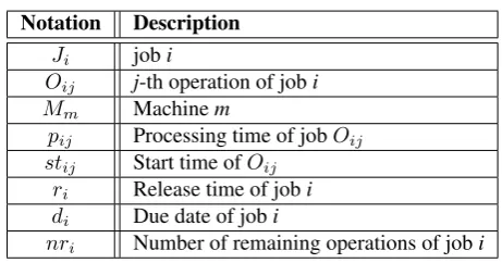
[image:2.595.179.410.545.666.2]

Some of the notations used to represent the jobs, machines and their features are summarized in Table 1.

Table 1.Notations

Notation Description

Ji jobi

Oij j-th operation of jobi

Mm Machinem

pij Processing time of jobOij

stij Start time ofOij

ri Release time of jobi

di Due date of jobi

nri Number of remaining operations of jobi

(3)

3 Previous Studies

[image:3.595.166.429.156.327.2]

It is important to understand the space of the methods search on to find an effective solution. Actually, for an effective search, the algorithms should search in different classes of the schedules. As seen in Figure 1, schedules are classified as (i) feasible, (ii) semi-active, (iii) active, and (iv) non-delay schedules [28][29].

Figure 1.Classification of the schedules [18][28]

A feasible schedule is a semi-active one if there isn’t any job or operation that can begin to process earlier without changing the order of the operations on any of the machines. An active schedule cannot be changed to another schedule in which any operation starts earlier, even by changing the order of operations on the machines. It is possible to obtain more than one active schedule in a scheduling problem. A feasible schedule is called non-delay if no machine is kept idle while an operation is waiting for processing [18]. Optimization methods that search for the optimal solution by creating the semi-active and active schedules are generally complex. So, in real problems of the manufacturing systems, the non-delay schedule generation by PRs can be a good approach [26][27]. Bierwirth has designed a heuristic that is applicable for both static and dynamic JSSPs with some modifications, which can be considered as a summary of the scheduling with PRs. In the JSSP, the technological order of a job, which defines the route that it must proceed, can be defined as Equation 2 [5].

τi= (Oiφi(1), ..., Oiφi(mi)) (2)

where,φi(k) =j, mi ≤m, 1≤k≤mimeans that thej-th operation of jobiis processed on the machinek. Based on

this definition, a none-delay schedule can be achieved with Equation 3.

stiφi(k)=

max(stiφi(k−1)+piφi(k−1), stlφl(k)+plφl(k))

1≤i, l≤n, 1≤k≤m

(3)

where,lis index of the job that processed before jobion machinek. The first part of the equation stands for the finish time of the next operation of jobi, while the second part shows the finish of the previous operation on machinek. Similarly, in a shop wherein the scheduling is done using a PR, when a machine is ready, a job is selected from the queue using a rule. The start time of each job on the related machine is the maximum of its own enter time to the queue and the time when the machine is free. This process can be easily applied as it is not complicated. In this way, PRs are used for sequencing the jobs that are waiting in the queue. Therefore, numerous studies are about PRs in the literature, which are often suggested to apply in real-time manufacturing systems. But no one of the rules in the literature is known to be globally better than the others. Because their efficiency depends on the characteristics of the system and the objective functions [14]. Many researchers have proposed new methods for extracting robust rules or have attempted to design them for specific environments [4][10][20][25].

(4)

two-phase learning method, that at first learns which part of the data correspond to best scheduling practices and then use this information in a decision tree to find new PRs [17]. Nie et al., have suggested a gene expression programming (GEP) based approach to generate PRs for solving a dynamic JSSP [15].

Kouiss et al. have proposed a multi-agent architecture for the dynamic scheduling problems, in which each agent represents a work center of a manufacturing system [12]. Hybrid methods based on the fuzzy precedence and decision-making models are also used for the dynamic scheduling problems. Subramaniam et al. have proposed an analytic hierarchy process (AHP) based dynamic scheduling method that selects a proper PR for each decision time according to the shop floor state [23]. In recent years, also the hyper-heuristics have been used frequently for applying the PRs dynamically [16].

4 The Proposed Algorithm

[image:4.595.168.428.359.484.2]

During the scheduling, when a machine is free, using a PR, one of the jobs waiting in the queue is selected and starts to process, and the other jobs wait until this process finishes. In this way, the waiting jobs are sequenced on the machines. In some study, the same rule is applied to all machines of the shop, while some others use a different rule for each machine. Another approach is to use different rules at each decision time, which is when a machine is empty, to select a job from the queue. In our approach, at first, it is necessary to divide the scheduling time into different intervals and define a PR for each of them. This scheduling policy is extracted using a simulation model combined with a GA. As seen in Figure 2, each chromosome, which is a scheduling policy, consists of two parts.

Figure 2.The chromosome of the GA

The first part contains the thresholds used to generate the intervals based on length of the queue (QL) and also based on the normalized processing times of the jobs waiting in the queues (P˜), which is calculated as Equation 4.

˜

P = p¯−pmin pmax−pmin

(4) where, p¯,pmax andpmin are the average, maximum and minimum processing times of the waiting jobs in the queue,

re-spectively. Based on the chromosome illustrated in Figure 2, based on QL, the queue of a machine is divided into 3 intervals as Equation 5.

0≤QL <X1

X1≤QL <X1+X2

X1+X2≤QL

(5)

In a similar way, as it is in Equation 6, the queue is divided into 3 intervals, according toP˜.

0≤P <Y˜ 1

Y1≤P <Y˜ 1+Y2

Y1+Y2≤P˜

(5)

Thus, totally3×3 = 9intervals are formed and using the second part of the chromosome, which corresponds to the rules, a policy as Equation 7 is obtained.

IF 0≤QL < X1 AND



 

 

0≤P < Y˜ 1, THEN R1

Y1≤P < Y˜ 1+Y2, THEN R2

Y1+Y2≤P ,˜ THEN R1.

IF X1≤QL < X1+X2 AND



 

 

0≤P < Y˜ 1, THEN R3

Y1≤P < Y˜ 1+Y2, THEN R1

IF X1+X2≤QL AND



 

 

0≤P < Y˜ 1, THEN R3

Y1≤P < Y˜ 1+Y2, THEN R1

(7)

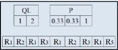
[image:5.595.152.441.153.291.2]

As seen in Figure 3, the thresholds for QL are integers, while they are decimal forP˜.

Figure 3.An example a chromosome as a scheduling policy

[image:5.595.198.397.352.437.2]

The classic rules used for the policy extraction are summarized in Table 3.

Table 2.Simple PRs used in the GA for scheduling policy extraction

Rule Assigned priority to jobi(Zi)

First In First Out (FIFO) ri

Shortest Processing Time (SPT) pij

Earliest Due Date (EDD) di

Least Remaining Operations Number (LRnOps) nri

(6)

[image:6.595.82.516.88.190.2]

Figure 4.Corresponding rules to the genes of the chromosomes

[image:6.595.197.398.305.417.2]

To apply the crossover, at first, a point is selected from the second part of the chromosome that contains the rules, which must be selected from the positions that correspond to the intervals that are generated according to the QL. For the chromo-some depicted in Figure 3, these points are shown in Figure 5. Then as it is done in the single-point crossover, the rules are exchanged. But also the thresholds that correspond to them are also changed. To apply the mutation, a new value is assigned to each gene, with a possibility equal to the mutation rate. which causes to changes in both the first and second part the chromosome.

Figure 5.The possible points for the crossover

The new population is also sent to the simulation where the fitness values of the chromosomes, i.e. the scheduling policies, are computed similarly to the process that is done for the initial population. This loop continues until the last iteration of the GA, which is the stop criterion. The extracted rule from the best chromosome of the last population is selected as the best scheduling policy.

5 Experimental Results

For the policy extraction and also to evaluate the performance, 82 problems have been selected from the abz5-abz9, ft06, ft10, and ft20, la01-la40, orb01-orb10, swv01-swv20 and yn1-yn4 test problems [1]. Due date of the jobs are assigned according to Equation 8 [25].

di= 2× ni X

j=1

pij (8)

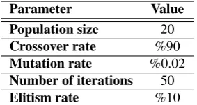
The parameters of the designed GA are in Table 3.

Table 3.Parameters of the proposed GA

Parameter Value

Population size 20

Crossover rate %90

Mutation rate %0.02

Number of iterations 50

[image:6.595.225.367.704.780.2]

(7)

[image:7.595.177.446.541.790.2]

The intervals and their thresholds are generated based on the parameters that are summarized in Table 4. They have been chosen experimentally, based on the results of the simulation model.

Table 4.Parameters of the interval and threshold generation

Number of thresholds for QL The distribution for generating thresholds for QL Number of the thresholds for P

3 Uniform(1,3) 4

3 Uniform(1,5) 4

2 Uniform(1,3) 4

2 Uniform(1,5) 4

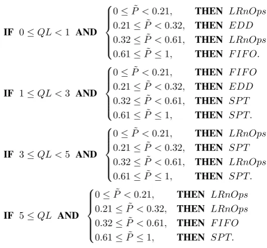
After 50 iterations, 4 scheduling policies as Equations 9, 10, 11 and 12 are generated.

Rule 1:

IF 0≤QL <1 AND



   

   

0≤P <˜ 0.21, THEN LRnOps 0.21≤P <˜ 0.32, THEN EDD

0.32≤P <˜ 0.61, THEN LRnOps 0.61≤P˜ ≤1, THEN F IF O.

IF 1≤QL <3 AND



   

   

0≤P <˜ 0.21, THEN F IF O 0.21≤P <˜ 0.32, THEN EDD

0.32≤P <˜ 0.61, THEN SP T 0.61≤P˜ ≤1, THEN SP T.

IF 3≤QL <5 AND



   

   

0≤P <˜ 0.21, THEN LRnOps 0.21≤P <˜ 0.32, THEN SP T

0.32≤P <˜ 0.61, THEN LRnOps 0.61≤P˜ ≤1, THEN SP T.

IF 5≤QL AND



   

   

0≤P <˜ 0.21, THEN LRnOps 0.21≤P <˜ 0.32, THEN LRnOps

0.32≤P <˜ 0.61, THEN F IF O 0.61≤P˜≤1, THEN SP T.

(8)

Rule 2:

IF 0≤QL <1 AND

        

0≤P <˜ 0.065, THEN LRnOps

0.065≤P <˜ 0.17, THEN F IF O 0.17≤P <˜ 0.54, THEN LRnOps

0.54≤P˜ ≤1, THEN F IF O.

IF 1≤QL <4 AND

        

0≤P <˜ 0.065, THEN SP T

0.065≤P <˜ 0.17, THEN LRnOps

0.17≤P <˜ 0.54, THEN SP T 0.54≤P˜ ≤1, THEN SP T.

IF 4≤QL <5 AND

        

0≤P <˜ 0.065, THEN EDD 0.065≤P <˜ 0.17, THEN EDD

0.17≤P <˜ 0.54, THEN EDD 0.54≤P˜ ≤1, THEN SP T.

IF QL≤5 AND

        

0≤P <˜ 0.065, THEN LRnOps 0.065≤P <˜ 0.17, THEN LRnOps

0.17≤P <˜ 0.54, THEN LRnOps 0.54≤P˜ ≤1, THEN EDD.

(10)

Rule 3:

IF 0≤QL <2 AND

        

0≤P <˜ 0.071, THEN EDD 0.071≤P <˜ 0.27, THEN F IF O

0.27≤P <˜ 0.54, THEN SP T 0.54≤P˜ ≤1 THEN SP T.

IF 2≤QL <4 AND

        

0.27≤P <˜ 0.54, THEN SP T

0.54≤P˜ ≤1 THEN EDD.

IF 4≤QL AND

        

0≤P <˜ 0.071, THEN F IF O 0.071≤P <˜ 0.27, THEN LRnOps

0.27≤P <˜ 0.54, THEN SP T

0.54≤P˜ ≤1 THEN EDD.

(11)

Rule 4:

IF 0≤QL <3 AND

        

0.76≤P <˜ 0.92, THEN SP T 0.92≤P˜ ≤1, THEN EDD.

IF 3≤QL <5 AND

        

0≤P <˜ 0.33, THEN F IF O 0.33≤P <˜ 0.76, THEN SP T

0.76≤P <˜ 0.92, THEN F IF O 0.92≤P˜ ≤1, THEN EDD.

IF 5≤QL AND

        

0≤P <˜ 0.33, THEN LRnOps 0.33≤P <˜ 0.76, THEN F IF O

0.76≤P <˜ 0.92, THEN F IF O 0.92≤P˜≤1, THEN SP T.

(9)

[image:9.595.89.506.133.348.2]

The convergence of the GA forRule 3is shown in Figure 6, which proves that it has reached the stable condition. Similar states are valid for the other rules.

Figure 6.The convergence of the GA forRule 3

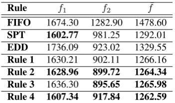
[image:9.595.42.563.424.546.2]

The performance of the obtained scheduling policy has been compared with the FIFO, SPT and EDD rules. The results are summarized in Figure 7 and Table 5.

Figure 7.The obtained results by the rules according to the (a) makespan, (b) mean flow time and (c) the defined objective function. In the figure, rules are as (1) FIFO, (2) SPT, (3) EDD , (4) Rule 1, (5) Rule 2, (6) Rule 3 and (7) Rule 4.

Table 5.Comparison between the extracted policies and some classical rules

Rule f1 f2 f¯

FIFO 1674.30 1282.90 1478.60

SPT 1602.77 981.25 1292.01

EDD 1736.09 923.02 1329.55

Rule 1 1630.21 902.11 1266.16

Rule 2 1628.96 899.72 1264.34

Rule 3 1636.30 895.65 1265.98

Rule 4 1607.34 917.84 1262.59

[image:9.595.209.385.620.723.2]

(10)

however, it is designed using the bigger thresholds for QL than Rules 1 and 3. It also has the second-best performance according tof1. However SPT provides the best makespan, all of the extracted rules have also good results according to this objective function. Generally, FIFO gets good results according to the makespan objective function, but it has a poor performance, which is due to the structure of the problem. For this objective function, EDD has the worst results, while this rule has achieved a fair mean flow time. FIFO has the worst results according to this objective function. According tof¯, among the classic rules, SPT has achieved the best result, while FIFO is the worst one. Although all of the designed rules have obtained similar results for this objective function, the best first 3 rules are Rules 4, 2, and 3, respectively.

6 Conclusion and Future Works

PRs are practical and useful methods to generate non-delay solutions for solving real scheduling problems. The dynamic and composite rules can achieve good results because they use more than one attribute. During the scheduling, the state of the queues change, so the jobs should be sequenced on the machines according to different features in each decision-making time. Although, in general, PRs can achieve fair results in all scheduling problems, the structure of the problem often affects the results. Therefore, it is a better approach to design the rules according to the problem or the manufacturing environment. It is clear that the rules should be easy to use. Usually, the dynamic rules can be easily implemented and also most of them are more efficient than the static rules.

Sometimes using too many rules can decrease the efficiency. It is possible to make better scheduling by choosing only the effective features, which corresponds to use less PRs. Also, the number of intervals for each feature affects the results. Such that in some problems, fewer intervals can provide good results, while in some others it should be more. It can be defined based on the results of an initial simulation, although, the evolutionary methods such as the Genetic Programming (GP) may be more useful for this aim. Another important matter that must be considered is that it is necessary to design the PRs according to the objective function of the problem. As it is observed in this study, a rule can achieve different results according to the different objective functions.

In this study, based on this approach and using different experimental parameters for generating intervals, 4 PRs are extracted, which are defined as IF-THEN. The results show that all of them provide the best results for the defined multi-objective function. Also, they have good results according to the single-objective functions. The Rule-4 that has the best results according to the multi-objective function, is generated with fewer intervals for QL. However, its thresholds are created at a larger interval than the Rules 1 and 3. The PRs and the proposed approach can be also applied to similar scheduling problems in manufacturing systems. In future work, we plan to design an agent-based scheduling algorithm for solving the dynamic JSSP with fuzzy processing times.

REFERENCES

[1] Or-library. http://people.brunel.ac.uk/~mastjjb/jeb/info.html. Accessed: 2018-02-20.

[2] J. Adams, E. Balas, and D. Zawack. The shifting bottleneck procedure for job shop scheduling. Management science, 34(3):391–401, 1988.

[3] D. Applegate and W. Cook. A computational study of the job-shop scheduling problem. ORSA Journal on computing, 3(2):149–156, 1991.

[4] O. Bahadir, G. Ozturk, and A. Teymourifar. Extracting new dispatching rules for dynamic multi-objective scheduling problems using simulation and gep. In3 rd INTERNATIONAL RESEARCHERS, STATISTICIANS AND YOUNG STATIS-TICIANS CONGRESS 24-26 MAY 2017 SELÇUK UNIVERSITY, 2017.

[5] C. Bierwirth, H. Kopfer, D. C. Mattfeld, and I. Rixen. Genetic algorithm based scheduling in a dynamic manufacturing environment. InEvolutionary Computation, 1995., IEEE International Conference on, volume 1, page 439. IEEE, 1995. [6] J. H. Blackstone, D. T. Phillips, and G. L. Hogg. A state-of-the-art survey of dispatching rules for manufacturing job shop

operations. The International Journal of Production Research, 20(1):27–45, 1982.

(11)

[8] O. Holthaus and C. Rajendran. Efficient dispatching rules for scheduling in a job shop.International Journal of Production Economics, 48(1):87–105, 1997.

[9] B.-W. Hsieh, S.-C. Chang, and C.-H. Chen. Dynamic scheduling rule selection for fab operations. InSemiconductor Manufacturing Technology Workshop, 2000, pages 202–210. IEEE, 2000.

[10] M. Jayamohan and C. Rajendran. Development and analysis of cost-based dispatching rules for job shop scheduling.

European Journal of Operational Research, 157(2):307–321, 2004.

[11] M. Kapanoglu and M. Alikalfa. Learning if–then priority rules for dynamic job shops using genetic algorithms. Robotics and Computer-Integrated Manufacturing, 27(1):47–55, 2011.

[12] K. Kouiss, H. Pierreval, and N. Mebarki. Using multi-agent architecture in fms for dynamic scheduling. Journal of Intelligent Manufacturing, 8(1):41–47, 1997.

[13] S. Lawrence. Resource constrained project scheduling: an experimental investigation of heuristic scheduling techniques (supplement).Graduate School of Industrial Administration, 1984.

[14] W. Mouelhi-Chibani and H. Pierreval. Training a neural network to select dispatching rules in real time. Computers & Industrial Engineering, 58(2):249–256, 2010.

[15] L. Nie, L. Gao, P. Li, and X. Shao. Reactive scheduling in a job shop where jobs arrive over time. Computers & Industrial Engineering, 66(2):389–405, 2013.

[16] G. Ochoa, J. A. Vázquez-Rodríguez, S. Petrovic, and E. Burke. Dispatching rules for production scheduling: a hyper-heuristic landscape analysis. InEvolutionary Computation, 2009. CEC’09. IEEE Congress on, pages 1873–1880. IEEE, 2009.

[17] S. Olafsson and X. Li. Learning effective new single machine dispatching rules from optimal scheduling data.International Journal of Production Economics, 128(1):118–126, 2010.

[18] M. L. Pinedo.Scheduling: theory, algorithms, and systems. Springer Science & Business Media, 2002.

[19] X. Qiu and H. Y. Lau. An ais-based hybrid algorithm with pdrs for multi-objective dynamic online job shop scheduling problem.Applied Soft Computing, 13(3):1340–1351, 2013.

[20] C. Rajendran and O. Holthaus. A comparative study of dispatching rules in dynamic flowshops and jobshops. European journal of operational research, 116(1):156–170, 1999.

[21] A. Shahzad and N. Mebarki. Data mining based job dispatching using hybrid simulation-optimization approach for shop scheduling problem. Engineering Applications of Artificial Intelligence, 25(6):1173–1181, 2012.

[22] R. Storer, S. Wu, and R. Vaccari. New search spaces for sequencing instances with application to job shop 38 (1992) 1495–1509manage. Sci, 38:1495–1509, 1992.

[23] V. Subramaniam, G. Lee, G. Hong, Y. Wong, and T. Ramesh. Dynamic selection of dispatching rules for job shop schedu-ling. Production planning & control, 11(1):73–81, 2000.

[24] E.-G. Talbi.Metaheuristics: from design to implementation, volume 74. John Wiley & Sons, 2009.

[25] J. C. Tay and N. B. Ho. Evolving dispatching rules using genetic programming for solving multi-objective flexible job-shop problems. Computers & Industrial Engineering, 54(3):453–473, 2008.

[26] A. Temourifar and G. Ozturk. New dispatching rules and due date assignment models for job shop scheduling problems.

Accepted to International Journal of Manufacturing Research, 2017.

[27] A. Teymourifar and G. Ozturk. A hybrid pareto-based swarm optimization algorithm for the multi-objective flexible job shop scheduling problems. World Academy of Science, Engineering and Technology, International Journal of Mechanical and Industrial Engineering, 4(7), 2017.

[28] A. Teymourifar and G. Ozturk. A neural network-based hybrid method to generate feasible neighbors for flexible job shop scheduling problem. Universal Journal of Applied Mathematics, 6(1):1–16, 2018.

(12)

[30] W. Xia and Z. Wu. An effective hybrid optimization approach for multi-objective flexible job-shop scheduling problems.

Computers & Industrial Engineering, 48(2):409–425, 2005.

[31] T. Yamada and R. Nakano. A genetic algorithm applicable to large-scale job-shop problems. InPPSN, pages 283–292, 1992.