The Constructive Implicit Function Theorem and Proof in Logistic Mixtures

(1)

The Constructive Implicit Function Theorem and Proof

in Logistic Mixtures

Xiao Liu

Methods in Empirical Educational Research, TUM School of Education and Centre for International Student Assessment (ZIB), TU M¨unchen, Arcisstr. 21, 80333 Munich, Germany

Abstract

There is the work by Bridges et al (1999) on the key features of a constructive proof of the implicit function theorem, including some applications to physics and mechanics. For mixtures of logistic distributions such information is lacking, although a special instance of the implicit function theorem prevails therein. The theorem is needed to see that the ridgeline function, which carries information about the topography and critical points of a general logistic mixture problem, is well-defined [2]. In this paper, we express the implicit function theorem and related constructive techniques in their mul-tivariate extension and propose analogs of Bridges and colleagues’ results for the mulmul-tivariate logistic mixture setting. In particular, the techniques such as the inverse of Lagrange’s mean value theorem [4] allow to prove that the key concept of a logistic ridgeline function is well-defined in proper vicinities of its arguments.

Keywords

Constructive Implicit Function Theorem, Logistic Mixture, Lagrange Mean Value Theorem, Ridgeline

1 Introduction

In this paper, we focuse on constructive techniques that are based on expressing the proof of implicit function theorem in their multivariate extension and propose analogs of Bridges and colleagues’ results for the multivariate logistic mixture setting.

According to [2], applying the implicit function theorem, we can prove that a unique explicit formula for the ridgeline function is possible locally in Theorem 1; In this paper, we propose analogs of Bridges et al.’s results (see [1]) for the multivariate logistic distribution.

Applying Lagrange’s mean value theorem (see [4]), we can get the first lemma. Moreover, we are interested in uniform differentiability of 2 variables on Lemma 3 due to [5], which carries important information about the proof of our goal.

2 Applications to Topography

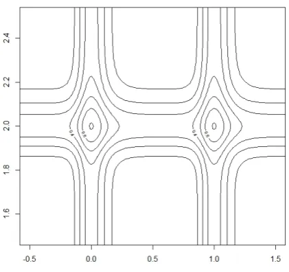
Theorem 1 later frequently allows us to show some ridgeline and contour plots, where the ridgeline function satisfies that the left side of formula (1) is equal to null (see [3]). The following example is in the case of two dimensions and three components.

Example 1. The mixture logistic density withD= 2andK= 3, and the parameters

µ₁=

(

0 0

)

, s1=

(

1 0.07

)

,

µ₂=

(

1 1

)

, s2=

(

0.07 1

)

,

µ₃=

(

2 2

)

, s3=

(

1 0.07

)

, π1=π2=π3=

1 3.

(2)

[image:2.595.200.411.87.285.2]

Figure 1.Density contour plot for the three component mixture density of Example 1.

3 The Constructive Implicit Function Theorem

For the most part we confine our attention to the following special case of the Implicit Function Theorem.

Theorem 1. Let

ψ(α,x) := K

∑

i=1

αi D

∑

k=1

s−_ik1

(

1−D+ 1 Eik

)

(1)

whereEik= 1 + e

xk−µik sik _{+ e}xk

−µik sik ∑D

j̸=ke

−xj_sij−µij_,

be a differentiable mapping of a neighbourhood of(α0,x0)∈RK×RDintoRp, letψ(α0,x0) = 0, and letdet(D2ψ(α0,x0))̸=

0. Then there existsr > 0and a differentiable functionf : ¯B(α0, r) ⊂ RK → RDsuch that for eachα ∈ B(α¯ 0, r),

(α, f(α))is the unique solutionxof the equationψ(α,x) = 0in some neighbourhood of(α0,x0).

Where we use standard modern notations for derivatives, such as Dfor the derivative itself, andDlfor thelth partial derivative (l= 1,2), of a mapping from a subset ofRK×RDtoRp.

This result, given here for the logistic mixture case, has obvious generalizations to any general implicit function as following corollary. To keep the presentation short we refrain from presenting them here, as their treatment follows the same strategy analogously to [1].

Corollary 1. Letψbe a differentiable mapping of a neighbourhood of(x0, y0)∈RK×RDintoRp, letψ(x0, y0) = 0, and

letdet(D2ψ(x0, y0))̸= 0. Then there existsr >0and a differentiable functionf : ¯B(x0, r)⊂RK →RDsuch that for

eachx∈B(x¯ 0, r),(x, f(x))is the unique solutionyof the equationψ(x, y) = 0in some neighbourhood of(x0, y0).

In next section, we will give the proof of Theorem 1. At last, we will show some necessary lemmata for preparing the proof of our main theorem in appendix.

4 A New Proof of The Constructive Implicit Function Theorem in The Case of

Logistic Mixtures

4.1

Proof of Theorem 1

Proof.

(i) Suppose that the assumption of Theorem 1 are satisfied, and chooser, s >0as in Lemma 2. Assume J :=B×C={(α,x) :|α−α0| ≤r,|x−x0| ≤s},

which is a compact set.

Fixξwith|ξ−α0| ≤r, and there∃ε >0such that

0< ε < m≡ inf

|h|≤r,|g|≤s|

(3)

Considerx,x∗such that|x−x0| ≤s,|x∗−x0| ≤s,and|ψ(ξ,x)−ψ(ξ,x∗)|< ε .

If|x−x∗| ≥ε, then due to Lemma 1,∃ηbetweenxandx∗such that

|D2ψ(ξ,η)| ≤ |x−x∗|−1ε2≤ε < m≤ |D2ψ(ξ,η)|, (3)

a contradiction. Thus|x−x∗|< ε.

In particular, if|ψ(ξ,x)|< ε2_and_|_ψ(ξ,_x∗₎_|_{< ε}2_{, then}_|_x₋_x∗_|_<_2ε.

(ii) Next give a hypothesis of that

0< γ:= inf

|x−x0|≤s

|ψ(ξ,x)|. (4)

If|x−x0| ≤s, then

|D2ψ2(ξ,x)|= 2|ψ(ξ,x)||D2ψ(ξ,x)| ≥2γm >0. (5)

According to the functionD2ψ2(ξ,·)is continuous on the segment

C := [x0−m,x0+m], without loss of generality, the Intermediate Value Theorem (see [4], Ch. 2) allows us to suppose

thatD2ψ2(ξ,x)≥2γmfor∀x∈C.

This implies thatψ2_(ξ,_·₎_{is strictly increasing on}_{C, and hence}_ψ2_(ξ,_x

0)> ψ2(ξ,x0−m); this is contradictory due to (12)

in view of the choice ofsin Lemma 2.

Thereforeγ= 0, then we can choosexnfor eachnsuch that|xn−x0| ≤sand|ψ(ξ,xn)|< 1

n2. Now the work in part (i)

of this proof shows that∃N, such that whennj, nl> N, we can get|xn_j −xn_l|< 2

n; then the sequence{xn}is a Cauchy sequence, and hence converges to a limitx_∞on the segmentC= [x0−m,x0+m]. The same argument shows thatx_∞is

also the unique solutionxonCof the equationψ(ξ,x) = 0, thus we can define a functionf : [α0−n, α0+n]→Cdue

tof(ξ) =x_∞.

On account of Lemma 3, we complete the proof.

A

Definition of Uniform Differentiability in 2 Variables

Definition 1. Letf :Rm_×_Rn_→_R_{be differentiable and such that}_∇_f_{is uniformly continuous. We define that}_f_{is uniformly} differentiable, i.e., for anyε >0, there is aδ >0such that for alla, x∈Rmandb, y∈Rn, we have

|f(a, b)−f(x, y)−D1f(x, y)(a−x)−D2f(x, y)(b−y)|

∥(a, b)−(x, y)∥ < ε

whenever∥(a, b)−(x, y)∥:=√∥a−x∥2₊_∥_b₋_y_∥2_{< δ.}

B

Three Lemmata

Although, logically unnecessary for the inverse of Lagrange’s Mean Value Theorem, it is, for pedagogical reasons, inter-esting to see that we show the following lemma. Moreover, the result will be also useful for the proof of Theorem 1.

Lemma 1. For every functionf :Rn_→_R_{with continuous partial derivatives}_f

x1,· · ·, fxnand for all distinct pairsaand

binRn_{, there exists an intermediate point}_x_{on the line segment joining}_a_and_b_{which we denote as}_x_∈_[a,_b]_{such that}

inf

x_∈[a,b]

|Df(x)| ≤ |b−a|−1|f(b)−f(a)|. (6)

Proof. According to [4], we can get

f(b)−f(a) =<b−a, Df(x)> (7)

then _⟨

b−a, inf

x∈[a,b]

|Df(x)|

⟩

≤ f(b)−f(a). (8)

Thus

inf

x_∈[a,b]

(4)

The following example of Lemma 1 can be applied for calculating the average velocity of non-uniform motion in kinematics.

Example 2. Let

f(x) =ax2+bx (a̸= 0) then

Df(x) = 2ax+b.

So we have

a(a+b−a)2+b(a+b−a)−aa2−ba = (b−a)

{

2a[a+1

2(b−a)] +b

}

.

The core to our mathematical expression of the existence of an implicit function in the logistic mixtures case is provided by the following lemma.

Lemma 2. Under the hypotheses of Theorem1, there existm∈RD_,_|_m_|₌_s,_n_∈_RK_,_|_n_|₌_{r, and}_{r, s >}₀_{such that}

|ψ(α0,x0±m)| ≥

2

3s|D2ψ(α0,x0)|, (10)

for∀h∈RK_,_g_∈_RD

inf

|h|≤r,|g|≤s|D2ψ(α0+h,x0+g)|>0, (11) and

inf

|h|≤r|

ψ(α0+h,x0±m)| ≥

1

2s|D2ψ(α0,x0)|>_|suph|≤r

|ψ(α0+h,x0)|. (12)

Proof. Choose an open ballB, with centre(α0,x0)and radiusR. Following formula (1), obviouslyD2ψ(α,x)∈ C0(B).

Then we can get

|D2ψ(α,x)|>

1

2|D2ψ(α0,x0)| (13)

for all(α,x)∈B.

According to thatψis differentiable at(α0,x0), there existss∈(0, R)such that if|x−x0| ≤s, we obtain

ψ(α0,x)−ψ(α0,x0)

x−x0

≤4

3|D2ψ(α0,x0)|, then

|ψ(α0,x)−D2ψ(α0,x0)(x−x0)| ≤

1

3|D2ψ(α0,x0)(x−x0)| (14) and therefore

|ψ(α0,x)| ≥

2

3|D2ψ(α0,x0)(x−x0)|. (15) In particular, choosex=x0±m, we obtain inequality (10). Sinceψ(α0,x0) = 0andψis continuous, we can now choose

r∈(0, R)such that inequality in (12) hold. According tor < R, our choice ofRensures that we can obtain inequality (11).

Next we separate out the proof of the differentiability of the implicit function. It will be convenient to establish the existence of Theorem 1 before.

Lemma 3.

LetBbe a compact ball inRK,Ca compact domain inRD, andψ:B×C→Rp_{be a uniformly differentiable function} such that

0< m:= inf

B×C|D2ψ|. (16)

Suppose that there exists a functionf :B →Csuch thatψ(α,x) = 0for∀α∈B, x:=f(α)∈C. Thenfis uniformly differentiable onB, and

f′(ξ) =−D1ψ(ξ, f(ξ))

D2ψ(ξ, f(ξ))

(5)

Proof. Let0< ε <₇m, and letα , α be points ofB, we define

∥α(1)−α(2)∥:=

√

ΣK i=1(α

(1)

i −α

(2)

i )2. (18)

According to Definition 1, we have the definition of uniform differentiability in 2 variables (also see [5]), so we can get

ψ(α(1), f(α(1)))−ψ(α(2), f(α(2)))−D1ψ

(

α(2), f(α(2))) (α(1)−α(2))

(19)

−D2ψ

(

α(2), f(α(2))) (f(α(1))−f(α(2)))

√

∥α(1)₋_α(2)_∥2₊_∥_f_(α(1)₎₋_f_(α(2)₎_∥2

≤ ε. Then ψ (

α(1), f(α(1))

)

−ψ

(

α(2), f(α(2))

)

(20)

−D1ψ

(

α(2), f(α(2))

) (

α(1)−α(2)

)

−D2ψ

(

α(2), f(α(2))

) (

f(α(1))−f(α(2)))

≤ ε

√

∥α(1)−_α(2)∥2₊∥_f_(α(1)₎−_f_(α(2)₎∥2

≤ ε(α(1)−α(2)+f(α(1))−f(α(2))

)

.

Otherwiseψ(α(1)_{, f}_(α(1)₎)₌_ψ(_α(2)_{, f}_(α(2)₎)_{= 0}_and_D 2ψ

(

α(2)_{, f}_(α(2)₎)_≥_m_{due to formula (16), so}

D1ψ

(

α(2), f(α(2)))

D2ψ

(

α(2)_{, f(α}(2)₎)

(

α(1)−α(2)

)

+f(α(1))−f(α(2))

≤ m−1ε(α(1)−α(2)+f(α(1))−f(α(2))

)

(21)

≤ 1

7

(_α(1)₋_α(2)₊_f(α(1)₎₋_f_(α(2)₎)_.

Therefore

f(α(1))−f(α(2))≤7

D1ψ

(

α(2)_{, f(α}(2)₎)

D2ψ

(

α(2)_{, f(α}(2)₎)

(

α(1)−α(2))+α(1)−α(2).

Choosing a boundM for|D1ψ|on the compact setB×C, we see that

f(α(1))−f(α(2))≤(7M m−1+ 1) α(1)−α(2). (22)

It follows from formula (21) that

D1ψ

(

α(2), f(α(2)))

D2ψ

(

α(2)_{, f(α}(2)₎)

(

α(1)−α(2)

)

+f(α(1))−f(α(2))

(23)

≤ m−1(7M m−1+ 2)εα(1)−α(2)→0

whenε→0.

Thusf is uniformly differentiable onB, with

f′(ξ) =−D1ψ(ξ, f(ξ))

D2ψ(ξ, f(ξ))

(6)

REFERENCES

[1] D. Bridges, C. Calude, B. Pavlov, D. Stefanescu. The Constructive Implicit Function Theorem and Applications in Mechanics, Chaos Solitons and Fractals, Vol.10, 927-934, 1999.

[2] X. Liu, A. ¨Unl¨u. Multivariate Logistic Mixtures, European Conference on Data Analysis (ECDA) , The University of Bremen, 105, 2014.

[3] X. Liu. Multivariate Logistic Mixtures, Universal Journal of Applied Mathematics, Vol.3, No.4, 77-87, 2015.

[4] P. K. Sahoo, T. Riedel. Mean Value Theorems and Functional Equations, World Scientific Press, New Jersey, 1998.