Bayesian Multiperiod Forecasting for Arma Model under Jeffrey's Prior

Bayesian Multiperiod Forecasting for Arma Model under

Jeffrey’s Prior

Zul Amry

1,*

_{, Adam Baharum}

2

1_{Department of Mathematics, State University of Medan, Indonesia} 2_{School of Mathematical Sciences, Universiti Sains Malaysia, Malaysia}

Copyright © 2015 by authors, all rights reserved. Authors agree that this article remains permanently open access under the terms of the Creative Commons Attribution License 4.0 International License.

Abstract

The main purpose of this study is to find the Bayesian forecast of ARMA model under Jeffrey’s prior assumption with quadratic loss function. The point forecast model is obtained based on the mean of the marginal conditional posterior predictive in mathematical expression. Furthermore, the point forecast model of the Bayesian forecasting compared to the traditional forecasting. The simulation shows that the forecast accuracy of Bayesian forecasting is better than the traditional forecasting and the descriptive statistics of Bayesian forecasting are closer to the true value than the traditional forecasting.

Keywords

ARMA Model, Bayes Theorem, Jeffrey’s Prior, Multiperiod Forecast

1. Introduction

The Bayesian approach in general requires explicit formulation of a model and conditioning on known quantities in order to draw inferences about unknown ones. The main difference between the Bayesian approach and the classical approach is that in the Bayesian approach, the parameters supposed as random variables, which are described by their probability density function, whereas the classical approach considers the parameters to be fixed but unknown. The classical forecasting has been developed by Box and Jenkins [4]. There are three steps are accomplished in the process of fitting the ARMA (p, q) model to a time series identification of the model, estimation of the parameters, and model checking to conclude whether the models obtained are adequate for forecasting. Several of works relating to Bayesian forecasting in the ARMA model are Fan & Yao [8] and Uturbey [13] using ARMA with normal-gamma prior. Kleibergen & Hoek [11], Liu [13], and Mohamed et al. [14] using ARMA model with Jeffrey's prior. This paper focuses on the Bayesian multiperiod forecasting for ARMA model using Jeffrey’s prior with quadratic loss function.

2. Materials and Methods

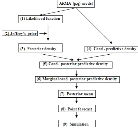
[image:1.595.312.549.421.643.2]

The materials in this paper are a set time series data in the ARMA model for application and simulation. The method is study of literature by applying a set of theories of mathematical statistics such as the ARMA model, likelihood function, Jeffrey’s prior, posterior distribution, Bayes theorem, conditional predictive density, conditional posterior predictive density, marginal conditional posterior predictive density, posterior mean and point forecast. Stages of discussion are presented in Figure 1 as follows:

Figure 1. Stages of discussion

3. Results

3.1. Likelihood Function

The one−step−ahead point forecast of yn+1 based data is

by:

)

|

(

)

1

(

ˆ

E

y

n ₁

S

n

y

=

+ (3.1)

This case is expandable for the k−step−ahead point forecast of yn + k, that is:

)

|

(

)

(

ˆ

* n k n

S

y

E

k

y

=

+ (3.2)

where

S

*_n= (y1, y2, …,yn+k-1)

The ARMA (p, q) model defined by:

∑

∑

= − = −

+

+

=

p i t q

j j t j i

t i

t

y

e

e

y

1 1

q

φ

(3.3)

where {et} is sequence of i i d normal random variables with

et∼N(0,t-1), t>0 and unknown, φi and qj are parameters.

Residuals are as:

∑

∑

= − = −

−

−

=

p i q

j j t j

i t i t

t

y

y

e

e

1 1

q

φ

(3.4)

By conditioning the first p observations and letting

ep=ep-1=…= er = 0, where r = min(0, p+1−q), one may

approximate ( Box & Jenkins, [4] ), the likelihood function for Ψ=(φ₁,φ_2, … ,φ_p, q₁, q₂, …, q_q) and t based

S

*_n is :

L (Ψ,t|

S

*_n) ∝t((n+k--p)|2

exp













































−

−

−

∑

+ −

∑

∑

+ = = − = − 1 1 2 1 1

2

k n p t q

j j t j

p

i i t i

t

y

e

y

φ

q

t

(3.5)

The equation (3.5) can be expressed as:

L (Ψ,t|

S

*_n) ∝t((n+k-1)-p)|2

(

)

1

1 1

2 1 ₂

1 1 1

1

exp

2

2

t t

n k n k

T _{n k}

t T

t p t p t

t p

y

y

_B

t

+ − + − −

+ −

= + = + −

= +





+













×

_

−

_

− Ψ

_

_

+

Ψ



_

_











∑

_{∑ ∑}

B

(3.6)

where Bt = (yt, yt-1, ..., yt+1-p, et, et-1, ..., et+1-q ) By allowing

U =





















































− − + − + − + − + − − + + − − + − + − − + + q k n q p q p k n p p k n p p p k n k n p p k n p p

e

e

e

e

e

e

e

e

e

y

y

y

y

y

y

y

y

y

1 2 1 3 1 2 1 1 2 1 3 1 2 1

ˆ

ˆ

ˆ

ˆ

ˆ

ˆ

ˆ

ˆ

ˆ

2









2

2

2









2

2

,

x0=

























− + + + 1 2 1 k n p p

y

y

y



, W=UU

T _{and V=Ux} 0

where

∑

∑

= − = −

−

−

=

p 1 i q 1 j j t j i

t i t

t

y

~

y

~

eˆ

eˆ

φ

q

, t = p+1, p+2, … , n,

i

~

φ

and

q

~

j are maximum likelihood estimator of

φ

i and

j

q

,

eˆ

_t

,

eˆ

_t−₁

,

2

,

eˆ

_t−_q be obtained via:

1

~

ˆ

=

−

T _t−

t

t

y

e

Ψ

B

(3.7) and the likelihood function can be expressed as:

L(Ψ,t |

S

*_n)

∝t((n+k-1)-p)|2





























+

−

−

∑

+ − + = 1 k n 1 p t T T 2

t

2

V

W

y

2

exp

t

Ψ

Ψ

Ψ

(3.8)

3.2. Posterior Distribution under Jeffrey’s Prior Assumption

Based the likelihood function in equation (3.8), the Jeffrey’s prior is:

1 1

Jeff

(

t

−

)

∝

t

−

π

(3.9)

By applying the Bayes theorem to equation (3.8) and (3.9), the posterior of

Ψ

and

t

−1 is:

π(Ψ,τ−1_|

* n

S

)∝ ( 1 2 ) 1 2

n k p p

t

+ − − + −

×

1 2 1

exp

2

2

n k T T t t p

W

V

y

t

+ −

= +













×

_

−

_

Ψ

Ψ − Ψ

+

_

_











∑



(3.10)

3.3. Conditional Predictive Density

Based on

∑

∑

= − = − − − = p 1 i q 1 j j t j i

t i t

t y y e

e

φ

q

with et∼ N(0,t-1),

be obtained:

(

)

[ ]











 −

=

− − − 2 t 2 1 1 1 * n

t

|

S

,

,

)

2

exp

₂

e

e

(

f

Ψ

t

πt

t

, if

expressed in yt as:

(

)

1

* 1 1 ₂

2

1 1

( | , , )

2

exp

2

t n

p q

t i t i j t j

i j

f y S

y

y

e

t

πt

t

_j

_q

−

− −

− −

= =

Ψ

=

×



_

_







×

_

−

_

−

−

_

_











∑

∑



, such

that the conditional predictive density of Yn+k based

Ψ

,

S

*

(

)

1

* 1 1 ₂

2

1 1

(

| , , )

2

exp

2

n k n

p q

n k i n k i j n k j

i j

f y

S

y

y

e

t

πt

t

_j

_q

−

− −

+

+ + − + −

= =

Ψ

=

×



_

_







×

_

−

_

−

−

_

_











∑

∑



∝

₂1

t

_                      + − −

∑

∑

= + − = + − + 2 p 1 i q 1 j j n k j i

k n i k

n y e

y 2

exp

t

φ

q

(3.11)

By changing

∑

∑

= + − = + −

+

p 1 i q 1

j j n k j i

k n

i

y

q

e

φ

to:

1 1 2 2

1 1 2 2

n k n k p n k p n k n k q n k q

y

y

y

e

e

e

j

j

j

q

q

q

+ − + − + −

+ − + − + −

+

+

+

+

+

+

+ +

2

2

=

(

)

                          − + − + − + − + − + − + q k n 2 k n 1 k n p k n 2 k n 1 k n q 2 1 P 2 1 e e e y y y   2

2 φ q q q

φ

φ ₌

1 k n T

_B

− +

Ψ

where ₁ 1 2

1 2

,

, ,

,

,

, ,

n k n k n k p

n k

n k n k n k q

y

y

y

B

e

e

e

+ − + − + − + − + − + − + −





=

_



_





2

2

, the

equation (3.11) can be written as:

)

,

,

S

|

y

(

f

* 1

n k

n+

Ψ

t

−

∝

_t

₂1

2 1

exp

2

y

n k T

B

n k

t

+ + −



_

_



×

_

−

_

− Ψ

_

_





∝

_t

₂1

[

]

_

  _{− − +} + − +

+

Ψ

Ψ

Ψ

t

_{y 2 B y R}

2 exp T k n 1 k n T 2 k n (3.12)

where

B

B

T

R

1 k n 1 k

n+ −

⊗

+ −

=

and

(

Ψ

TBn+k−1

)

2 =

Ψ

T R

Ψ

. 3.4. Conditional Posterior Predictive Density

Based equation (3.10) and equation (3.12) be obtained the conditional posterior predictive density:

)

,

,

S

|

y

(

f

* 1

n k n

p +

Ψ

t

−

∝

( 1 2 ) _{1 1} 2

n k p p

t

+ − − + + −

×

1 1 2 2 1 1

(

)

exp

(

)

2

T T

n k n k

n k

T T

n k n k n k t

t p

Z

V B

y

V

B

y

y

y

t

+ − +

+ −

+ − + +

= +





Ψ

Ψ − Ψ

+

−













×

_

−

_

_

_

+

Ψ +

+



_

_









∑



(3.13) where Z = W + R

3.5. Marginal Conditional Posterior Predictive Density The marginal conditional posterior predictive density of

Yn+k be obtained by integrating equation (3.13) with respect

to Ψ and t−1_{, that is:}

)

S

|

y

(

f

* n k n

p + =_{0 0}

f

(

y

|

S

,

Ψ

,

t

)

d

ψ

d

t

1 * n k n p

∫ ∫

∞ ∞ − +

(

)

(

)

1

2 2 1

1 1

( 1 2 ) _{1 1}

1 2

0

exp

2

n k _T

n k t n k n k n k n k

n k p p

t p

y

y

V B

y

Z V B

y

d

t

t

t

+ − − + + − + + − + ∞ + − − + + − _{= +}





₊

₋

₊

₊















_

_



∝

_

− ×

_







_

_





_

_







∑

∫

(3.14)

By using the formula of gamma-distribution, based equation (3.14) be obtained:

)

S

|

y

(

f

* n k n

p +

∝

(

) (

)

[

]

(

)

(

)

2 1 ) 1 ( 1 1 1 0 1 1 2 2 1 1 1 1 1 1 1 1 1 1 + − − + − − + − − + − + + = − − + − − + − − + +                                       − − − + − − − + − − +

∑

p k n k n T k n T k n p t t T k n k n T k n k n B Z B p k n V Z V y V Z B B Z B y p k

n (3.15)

The marginal conditional posterior predictive density of Yn+k is a univariate student’s t−distribution on (n+k−1−p) degrees

of freedom with mean

(

1

B

Z

B

) (

B

T

Z

1

V

)

.

1 k n 1 1 k n 1 T 1 k

n + − −

3.6. Point Forecast

For quadratic loss function, the point forecast of Yn+k is the

posterior mean of the marginal conditional posterior predictive, that is:

(

)

(

) (

)

* 1

1 1

1 1 1

ˆ( )

|

1

n k n

T T

n k n k n k

y k

E Y

S

B

Z B

B

Z V

+

−

− −

+ − + − + −

=

=

= −

(3.16)

4. Simulation

A simulation study was conducted to compare between the Bayesian forecasting and the traditional forecasting of the ARMA (1, 1) model with

φ

~

=0.93176 and

q

~

=0.56909 for series lengths of 70, 90, 110, 130, 150, 180. 210, 240, 270 and 300 each to forecast the 10 steps ahead. The result of forecast by using the traditional method is:

1 60 1 60

~

ˆ

ˆ

~

)

(

ˆ

k

=

y

+k−

+

e

+k−

y

φ

q

=

60 1 60 1

ˆ

ˆ

0.93176

y

+ −k

0.56909

e

+ −k

=

+

_(3.17)

where

eˆ

_k

=

yˆ

_k

−

0

.

93176

yˆ

_k−₁

−

0

.

56909

eˆ

_k−₁ ,

k=1,2,3, …, 10.

4.1. Comparison of Forecast Accuracy and Descriptive Statistics

There are measures to determine the accuracy of a forecasting model. Assis [1] in their paper present four measures, namely Root Mean square Error (RMSE), Mean Absolute Error (MAE), Mean Absolute Percentage Error (MAPE) and U-statistic defined respectively as follows:

n

ESS

RMSE

=

(3.18)

n

Y

Y

MAE

n

t t t

∑

=

−

=

1

ˆ

(3.19)

%

100

ˆ

1

x

n

Y

Y

Y

MAPE

n

t t

t t

∑

=

−

=

(3.20)

U-statistics=

∑

∑

= =

+

n

t n

t

n

Y

n

Y

RMSE

1 2 1

2

ˆ

(3.21)

where Yt = the factual value at time t,

Yˆ

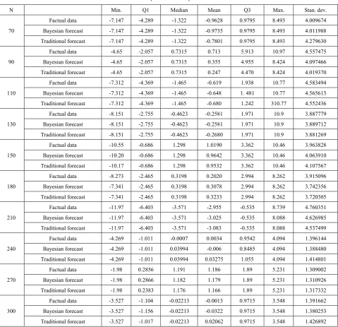
_t= the forecast value at time t, n= the number of observations, and ESS = the error sum of square.

[image:4.595.352.556.76.321.2]

The comparison of forecast accuracy between Bayesian method in equation (3.16) with traditional method in equation (3.17) is presented in the Table 1. The comparison of descriptive statistics is presented in the Table 2, Columns 3 through 9 contain the minimum (Min), first quartile (Q1), median, mean, third quartile (Q3), maximum (Max), and standard deviation for N factual data, N-10 factual data and the result of Bayesian forecasting for the 10 steps ahead, and N-10 factual data and the result of traditional forecasting for the 10 steps ahead.

Table 1. Comparison of forecast accuracy

N Bayesian Traditional

[image:5.595.66.546.83.546.2]

Table 2. Comparison of descriptive statistics

N Min. Q1 Median Mean Q3 Max. Stan. dev.

70

Factual data -7.147 -4.289 -1.322 -0.9628 0.9795 8.493 4.009674 Bayesian forecast -7.147 -4.289 -1.322 -0.9735 0.9795 8.493 4.011988 Traditional forecast -7.147 -4.289 -1.322 -0.7801 0.9795 8.493 4.279630

90

Factual data -4.65 -2.057 0.7315 0.713 5.913 10.97 4.557475 Bayesian forecast -4.65 -2.057 0.7315 0.355 4.955 8.424 4.097466 Traditional forecast -4.65 -2.057 0.7315 0.247 4.470 8.424 4.019370

110

Factual data -7.312 -4.369 -1.465 -0.619 1.938 10.77 4.583494 Bayesian forecast -7.312 -4.369 -1.465 -0.648 1. 481 10.77 4.565613 Traditional forecast -7.312 -4.369 -1.465 -0.680 1.242 310.77 4.552436

130

Factual data -8.151 -2.755 -0.4623 -0.2581 1.971 10.9 3.887779 Bayesian forecast -8.151 -2.755 -0.4623 -0.2581 1.971 10.9 3.889712 Traditional forecast -8.151 -2.755 -0.4623 -0.2680 1.971 10.9 3.881269

150

Factual data -10.55 -0.686 1.298 1.0190 3.362 10.46 3.963828 Bayesian forecast -10.20 -0.686 1.298 0.9642 3.362 10.46 4.063910 Traditional forecast -10.17 -0.686 1.298 0.9532 3.362 10.46 4.107567

180

Factual data -8.273 -2.465 0.3198 0.2020 2.994 8.262 3.915096 Bayesian forecast -7.341 -2.465 0.3198 0.3078 2.994 8.262 3.742356 Traditional forecast -7.341 -2.465 0.3198 0.3233 2.994 8.262 3.720305

210

Factual data -11.97 -6.403 -3.571 -2.955 -0.535 8.739 4.760351 Bayesian forecast -11.97 -6.403 -3.571 -3.025 -0.535 8.088 4.626985 Traditional forecast -11.97 -6.403 -3.571 -3.083 -0.535 8.088 4.537499

240

Factual data -4.269 -1.011 -0.0007 0.0034 0.9542 4.094 1.396144 Bayesian forecast -4.269 -1.011 0.03994 -0.006 0.8485 4.094 1.388480 Traditional forecast -4.269 -1.011 0.03994 0.03275 1.055 4.094 1.414801

270

Factual data -1.98 0.2856 1.191 1.186 1.89 5.231 1.309002 Bayesian forecast -1.98 0.2866 1.182 1.179 1.89 5.231 1.310926 Traditional forecast -1.98 0.2383 1.176 1.166 1.89 5.231 1.317332

300

Factual data -3.527 -1.104 -0.02213 -0.0013 0.9715 3.548 1.391662 Bayesian forecast -3.527 -1.156 -0.02213 -0.0322 0.9715 3.548 1.380253 Traditional forecast -3.527 -1.017 -0.02213 0.02062 0.9715 3.548 1.426892

5. Conclusions

The results in the Table 2 shows that the forecast accuracy value of the Bayesian method is smaller than the traditional method, it is indicates that the forecast accuracy the Bayesian forecasting is better than the traditional forecasting. The results in the Table 3 shows that descriptive statistics of Bayesian forecasting is closer to the factual data as compared to traditional forecasting, so it can be concluded that Bayesian forecasting is better than traditional forecasting.

REFERENCES

[1] Assis, K, Amran, A. and Remali, Y. (2010). Forecasting Cocoa Bean Prices Using Univariate Time Series Models.

Journal of Arts & Commerce. ISSN 2229-4686, Vol.- I, Issue-I, 71-80

[2] Bain, L.J. and Engelhardt, M.(1992). Introduction to Probability and Mathematical Statistics, 2nd_{. Duxbury Press,}

Belmont, California.

[3] Bijak, J. (2010). Bayesian Forecasting and Issues of Uncertainty. Centre for Population Change, University of Southampton, 1-19.

[4] Box, G.E.P. and Jenkins, G. M. (1976). Time Series Analysis: Forecasting and Control. Holden-Day, San Francisco. [5] Enders, W. (1995). Applied Econometric Time Series. John

Wiley & Son. Inc. New York.

[6] Faisal, F. (2012). Forecasting Bangladesh’s Inflation Using Time Series ARIMA Models. Paper.

Process and Its Application. International Business Research, 1(4), 49-55.

[8] Gelman, A. (2008), Objections to Bayesian statistics,

Bayesian Analysis 3(3), 445−450.

[9] Geweke, J and Whiteman, C., (2004), Bayesian Forecasting, Department of Economics, University of Iowa.

[10] Ihaka, R. (2005). Time Series Analysis. Statistics Department University of Auckland.

[11] Kleibergen, F. and Hoek, H. (1996). Bayesian Analysis of ARMA model Using Non informative Prior. Paper, Econometric Institute, Erasmus University, Rotterdam, 1−24

[12] Liu,S. I.(1995). Bayesian Multiperiod Forecasts for ARX Models. Ann. Inst. Statist. Math. Vol. 47, no.2,211-224.

[13] Liu,S.I.(1995). Comparison of Forecast sfor AR Models Between A Random Coefficient Approach and A Bayesian Approach. Commun Statist.- Theory Meth., 24(2), 319-333

[14] Mohamed, I., Zaharim, A. and Yahya M.S. (2002). Penganggaran Parameter bagi Model BL (p,0,1,1) dengan Pendekatan Bayesian. Matematika, jilid 18, bil. 2, hlm. 129-136, Jabatan Matematika UTM.

[15] Pole, A., West, M. and Harrison, J. (1994). Applied Bayesian Forecasting and Time Series Analysis. Chapman and Hall, New York.

[16] Ramachandran, K.M. and Tsokos, C.P. (2009).Mathematical Statistics with Applications, Elsevier Academic Press. San Diego, California.

[17] Salam, M.A., Salam, S., and Feridun, M. (2006). Forecasting Inflation in Developing Nations: The Case of Pakistan.

International Research Journal of Finance and Economics, ISSN 1450-2887, Issue 3, 138-159.

[18] Research Journal of Finance and Economics, ISSN 1450-2887, Issue 62, 111- 142

[19] Stovicek K. (2007). Forecasting with ARMA Models, The case of Slovenian Inflation, Prikazi in analize XIV/1, 23-45.

[20] Uturbey, W. (2006). Identification of ARMA Model by Bayesian Methods Applied to Streamflow Data. 9th International Conference on Probabilistic Method Applied to Power Systems KTH ( 11-15June 2006, Stockholm, Sweden ), 1-7