The General Two Dimensional Shifted Jacobi Matrix Method for Solving the Second Order Linear Partial Difference differential Equations with Variable Coefficients

The General Two Dimensional Shifted Jacobi

Matrix Method for Solving the Second Order

Linear Partial Difference-differential Equations

with Variable Coefficients

Z. Kalateh Bojdi

1

_,

_{S. Ahmadi-Asl}

1

_,

_{A. Aminataei}

2,∗

1_{Department of Mathematics, Birjand University, Birjand, Iran}

2_{Faculty of Mathematics, K. N. Toosi University of Technology, P.O. Box 16315-1618, Tehran, Iran} ∗_{Corresponding Author: [email protected]}

Copyright c⃝2013 Horizon Research Publishing All rights reserved.

Abstract

In this paper, a new and efficient approach for numerical approximation of second order linear partial differential-difference equations (PDDEs) with variable coefficients is introduced. Explicit formulae which express the two dimensional Jacobi expansion coefficients for the derivatives and moments of any differentiable function in terms of the original expansion coefficients of the function itself are given in the matrix form. The main importance of this scheme is that using this approach reduces solving the general linear PDDEs to solve a system of linear algebraic equations, wherein greatly simplify the problem. In addition, some experiments are given to demonstrate the validity and applicability of the method.

Keywords

General Two Dimensional Jacobi Matrix Method, Second Order Linear Pddes with Variable Coef-ficients

2010 AMS subject classifications: 35-XX, 33C45

1

Introduction

approximation of the second order linear PDDE (with the initial and boundary conditions which has a solution which is expressible as a known elementary function) in the following form

1

∑

j=0 1

∑

i=0

Pi,j(x, y) ∂

i+j

∂xi_∂yju(x+k, y+h) =g(x, y), a≤x≤b, a≤y≤b,

k, h∈Z,

(1)

where the coefficientsPk,j(x) andg(x, y) have the two dimensional Taylor series expansions and Zdenotes the set

of integer numbers. The main importance of our work is considering the general second order linear PDDE (1), wherein the other papers only considered particular cases of our general problem. Also using the general shifted Jacobi polynomials as the basic functions for numerical approximation wherein the shifted Chebyshev (first to fourth kinds) and Legendre polynomials are particular cases of them, is the other superiority of our paper. The remainder of this paper is organized as follows: In Section 2, we introduce the properties of the one and two dimensional shifted Jacobi polynomials and the basic formulation of them is required for our subsequent development. Section 3, is devoted to the operational matrix of the one and two dimensional shifted Jacobi polynomials (derivative and moment) with some useful theorems. Section 4, summarizes the application of the two dimensional shifted Jacobi matrix method to the solution of problem (1). Thus, a set of algebraic equations is formed and a solution of the considered problem is introduced. In Section 5, we present the approximation with Jacobi polynomials. In section 6, the proposed method is applied to the two numerical experiments. The applications of the new method for the high order linear PDDEs is presented in Section 7. Finally, we have monitored a brief conclusion in section 8. Note, that we have computed the numerical results by Matlab (version 2013) programming.

1.1

Preliminaries and notations

We first introduce some notations, which we use in the following.

Definition 1. A PDDE is a relation that involves partial derivatives of an unknown function. Let the unknown function beu,andx, y, ...be independent variables. i.e.,u=u(x, y, z, ...,).Often, one of these variables represents the time. Thus a PDDE is an equation of the form

F(x+h, y+k, z, u, ux, uy, uz, uxx, uxy, ..., uxxx, ...) = 0, (2)

wherehandk∈Z. In Eq.(2), we have used the subscript notation for the partial differentiation ux=

∂u

∂x, uxy= ∂2_u

∂x∂y, (3)

and so on. We will always assume that the unknown functionuis sufficiently well behaved so that all necessary partial derivatives exist and the corresponding mixed partial derivatives are equal, e.g.,

uxy=uyx, uxzx=uxxz, (4)

and so on.

Definition 2. As in the case of ordinary differential equations (ODEs), the order of the PDDEs is defined in Eq.(2), to be the highest order of partial derivatives appearing in the equation.

Definition 3. We say that the PDDE (2), is linear if F is linear as a function of the variablesux, uy, uz, uxx, ..., .

i.e.,F is a linear combination of the unknown function and its derivatives. Eq.(2) is said to be quasilinear ifF is linear as a function of the highest-order derivatives.

2

The one and two dimensional shifted Jacobi polynomials

The classical Jacobi polynomial of degree n, Jn(α,β)(z) [31-33] is defined on the interval [−1,1] and can be

determined with the aid of the following recurrence formulae:

J₀(α,β)(z) = 1, J₁(α,β)(z) =1₂(α+β+ 2) +1₂(α+β), J_n(α,β₊₁)(z) = (anz−bn)J

(α,β)

n (z)−cnJ

(α,β)

n₋1 (z), n≥1,

(5)

where

an =

(2n+α+β+1)(2n+α+β+2) 2(n+1)(n+α+β+1) ,

bn=

(2n+α+β+1)(β2_−α2₎

2(n+1)(n+α+β+1)(2n+α+β),

(6) and

cn=

(2n+α+β+ 2) (n+β)

For using the general shifted Jacobi polynomials on the interval [a, b], we shift the defining domain by means of the following substitution:

z=2x−a−b

b−a , a≤x≤b. (8)

These polynomials construct the orthogonal polynomials with respect to the weight functionw(α,β)_{(x) = (b−x)}α_(x−a)β_,

over [a, b]

∫ b

a

P_m(α,β)(x)P_n(α,β)(x)w(α,β)(x)dx=η_nα,βδmn, (9)

whereδmnis the Kronecker delta function and

η_nα,β=P_m(α,β)(x)

2

w(α,β)=

(b−a)α+β+2m−12α+β+2_{Γ(m+α+ 1)Γ(m+β+ 1)}

m! (2m+α+β+ 1) Γ(m+β+α+ 1) . (10) A functiony(x)∈L2

w(α,β)[a, b], can be expressed in terms of the general shifted Jacobi polynomials as

y(x) =

∞ ∑

i=0

aiP

(α,β)

i (x), (11)

where the coefficientai is given by

ai =

1 η_iα,β

∫ b

a

P_i(α,β)(x)y(x)w(α,β)(x)dx. (12)

In practice, only the firstm+ 1 terms of the shifted Jacobi polynomials are considered. Then we have

ym(x) = m

∑

i=0

aiP

(α,β)

i (x) =

(

P(α,β)(x)

)T

A, (13)

where the shifted Jacobi coefficient vectorAand the shifted Jacobi vectorP(α,β)_{(x) are given by}

A= [a0, a1, ..., am]T, (14)

and

P(α,β)(x) =

[

P₀(α,β)(x), P₁(α,β)(x), ..., P_m(α,β)(x)

]T

. (15)

Similarly a functionf(x, t) of the two independent variables is defined ona≤x, y≤b may be expanded in terms of the two dimensional shifted Jacobi polynomials as

fm(x, t) = m

∑

i=0

m

∑

j=0

ci,jP

(α,β)

i (x)P

(α,β)

j (y) =

(

P(α,β)(x)

)T

C

(

P(α,β)(y)

)

, (16)

where the shifted Jacobi coefficients matrixC is given by

C=

  

c11 . . . c1m

..

. . .. ... cm1 · · · cmm

 

, (17)

where

ci,j=

1 η_i(α,β)η_j(α,β)

∫ b

a

∫ b

a

f(x, y)P_i(α,β)(x)P_j(α,β)(y)wα,β(x)wα,β(y)dxdy, i, j= 1, ..., m. (18) Now in the following theorem, we present the explicit form of the shifted Jacobi polynomials.

Theorem 1. The explicit form of the shifted Jacobi polynomials are in the following form

P_n(α,β)(x) =

n

∑

i=0

G(_iα,β,n)xi; α, β >−1, (19)

where

G(_iα,β,n)=

n

∑

k=i

2k

(b−a)k

(−b)i−kB_k(α,β,n), (20) and

B_k(α,β,n)= 2−k

(

n+α+β+k k

) (n+α n−k

)

Proof. From [34], we have

J_n(α,β)(z) =

n

∑

i=0

B_i(α,β,n)(1−z)i; α, β >−1, (22) where

B_k(α,β,n)= 2−k

(

n+α+β+k k

) (n+α n−k

)

; k= 0,1,2, ..., n. (23)

Now using substitution of Eq.(8) into Eq.(22) yields Pn(α,β)(x) =J

(α,β)

n (2x_b−₋a_a−b) = n

∑

i=0

B(_iα,β,n)

(

2

b₋a

)i

(x−b)i=

n

∑

i=0

B_i(α,β,n) 2i

(b−a)i

i

∑

k=0

(_i

k

)

(−b)i−kxk_,

(24)

from Eq.(24) and defining

G(_iα,β,n)=

n

∑

k=i

2k

(b−a)k

(−b)i−kB_k(α,β,n), (25) the proof is completed.

Also from theorem 1, we can obtain the explicit form of the two dimensional shifted Jacobi polynomials as the following

P_n(α,β)(x)P_m(α,β)(y) =

n

∑

i=0

m

∑

j=0

G(_iα,β,n)G(_jα,β,m)xiyj, (26)

and from the two dimensional Taylor series, we can obtain the following formula

G(_iα,β,n)G(_jα,β,m)=∂

i+j_{f(x, y)}

∂xi_∂yj (0,0), (27)

where

f(x, y) =P_n(α,β)(x)P_m(α,β)(y). (28) From theorem 1, we can obtain the matrix relation between general shifted Jacobi polynomials space (set)

{P₀(α,β)(x), P₁(α,β)(x), ..., Pn(α,β)(x)}and standard polynomial space (set) as the following

[

P₀(α,β)(x), P₁(α,β)(x), ..., Pn(α,β)(x)

]T

=K[1, x, ..., xn]T, (29) whereK is a lower triangular matrix

(K)_i,j=

{

0, i > j,

G(_jα,β,i), i≤j. (30)

Theorem 2. The matrixKis invertible if and only ifα, β >0, which is a consequence of the fact that the matrix associted to a change of bases is always nonsingular.

Proof: For establishing the invertibility of matrixK,it is sufficient to show that

Det (K)̸= 0, (31)

where Det(K) is a determinant of the square matrixK. But because Kis a lower triangular matrix, then we have

Det (K) =

n

∏

i=0

G(_iα,β,i), (32)

and from (25) and (30), we have

G(_iα,β,i)=

i

∑

k=i

2k

(b₋a)k(−b)

i₋k

B_k(α,β,n)=

2i (b−a)i(−b)

i−i_B(α,β,i)

i =

2i (b−a)i2−

i

(

2i+α+β i

) (

i+α 0

)

=



 2i+α+β

i

 

(b₋a)i ̸= 0, ∀α, β >0,

(33)

Remark 1. From theorem 2, we conclude that in situations that we need the invertibility of matrixK,choosing parameters−1< α, β <0,is not suitable.

Now from (29), we can obtain the following important matrix relation, which is an immediate consequence of the above fact

[1, x, ..., xm]T =K−1

[

P₀(α,β)(x), P₁(α,β)(x), ..., P_m(α,β)(x)

]T

,∀α, β >0. (34)

3

Operational matrices of the two dimensional shifted Jacobi

polyno-mials (derivative, moment and shift)

In this section, we present the operational matrices of the general shifted Jacobi polynomials (derivative, shift and moment). The derivative and moment operational matrices with respect to the classical Jacobi polynomials are obtaind in [35] and we present them in the following theorems.

To do this, first we introduce the concept of operational matrix.

3.1

The operational matrix

Definition 4. Suppose

ϕ= [ϕ0, ϕ1, ..., ϕn], (35)

whereϕ0, ϕ1, ..., ϕn are the basis functions on the given interval [a, b]. The matricesEn×nandFn×n are named as

the operational matrices of the derivatives and integrals respectively if and only if

d

dtϕ(t)≃Eϕ(t),

∫x

a ϕ(t)dt≃F ϕ(t).

(36)

Further assumeg= [g0, g1, ..., gn],named as the operational matrix of the product, if and only if

ϕ(x)ϕT(x)≃Ggϕ(x). (37)

In other words, to obtain the operational matrix of a product, it is sufficient to findgi,j,k in the following relation

ϕi(x)ϕj(x)≃ i+j

∑

k=0

gi,j,kϕk(x), (38)

which is called the linearization formula [34]. Operational matrices are used in several areas of numerical analysis and they hold particular importance in various subjects such as integral equations [36], differential equations [37], integro-differential equations [38] and etc. Also many textbooks and papers have employed the operational matrices for spectral methods. Now we present the following theorem.

Theorem 3. If we consider the Jacobi approximation

y(x)∼=

m

∑

i=0

aiP

(α,β)

i (x) =

(

P(α,β)(x)

)T

A, (39)

then

xiy(j)(x)∼=BTP(α,β)(x) =((GiDj)TA

)T

P(α,β)(x), (40) where

D=

(

0 E−1

0 0

)

(n+1)×(n+1)

, Ep,q=

        

−2(p+α+1)(p+β+1)

(α+β+p+1)(α+β+2p+2)(α+β+2p+3), p=q−2, 2(α₋β)

(α+β+2p)(α+β+2p+2), p=q−1, 2(α+β+p)

(α+β+2p−1)(α+β+2p), p=q,

0, otherwise,

(41)

and

Gp,q =

        

2(p+α)(p+β)

(α+β+2p)(α+β+2p+1), p=q−1,

β2−α2

(α+β+2p+1)(α+β+2p+2), p=q, 2p(α+β+p)

(α+β+2p)(α+β+2p₋1), p=q+ 1,

0, otherwise.

(42)

Now by using theorem 1, we obtain the operational matrix for the following operator (the two dimensional case)

L(f(x, t)) =xiyj ∂ ∂xk_∂yd

(_m ∑ t=0 n ∑ p=0

at,pP

(α,β)

t (x)Pp(α,β)(y)

)

. (43)

For this goal, we present the following theorem.

Theorem 4. If we consider the Jacobi approximation (39) and the operator (43), then we have

xi_yj ∂k+d

∂xk_∂yd ( m ∑ t=0 n ∑ p=0

at,pP

(α,β)

t (x)P

(α,β)

p (y)

)

≃(P(α,β)_(x))T((_Dk)T(_Gi)T_AGj_Dd) (_P(α,β)_(y))₌

(

P(α,β)_(x))T(_A(i,j) (k,d)

) (

P(α,β)_(y))_.

(44)

Proof. If we consider the following relations

xiyj_∂x∂kk+_∂ydd ( m ∑ t=0 n ∑ p=0

at,pP

(α,β)

t (x)P

(α,β)

p (y)

)

=xiyj_∂xk∂_∂yd ((

P(α,β)(x))T(C)(P(α,β)(y)))= xi ∂k

∂xk (

P(α,β)_(x))T_(C)yj ∂d ∂yd

(

P(α,β)_(y))₌(_P(α,β)_(x))T((_Dk)T(_Gi)T_AGj_Dd) (_P(α,β)_(y))₌

(

P(α,β)_(x))T(_A(i,j)

(k,d)

) (

P(α,β)_(y))_,

(45)

the proof is completed.

Now we present a useful theorem which we need for obtaining the operational matrix with respect to the shift operator. This is also a consequence of the connection formula stated in theorem 1 as well as formula (34).

Theorem 5. Ifc∈R andα, β >0,then

[

P₀(α,β)(x+c), P₁(α,β)(x+c), ..., P_n(α,β)(x+c)

]T

=WcK−1

[

P₀(α,β)(x), P₁(α,β)(x), ..., P_n(α,β)(x)

]T

, (46) whereWc is a lower triangular matrix

(Wc)i,j=

{

0, i < j,

D(_iα,β,j), i≥j, (47)

and

D(_iα,β,j)=

j

∑

k=i

G(_kα,β,j)ck

(

k i

)

, (48)

andG(_kα,β,j) is defined in (25). Proof: From (19), we have

Pn(α,β)(x+c) = n

∑

i=0

G(_iα,β,n)(x+c)i=

n

∑

i=0

G(_iα,β,n)

i ∑ j=0 ( i j )

ci−j_xj_{, (49)}

so if we define

D_i(α,β,j)=

j

∑

k=i

G(_kα,β,j)ck

(

k i

)

, (50)

therefore we have

P_n(α,β)(x+c) =

n

∑

i=0

D(_iα,β,n)xi. (51)

Using obtained result (51), we have

[

P₀(α,β)(x+c), P₁(α,β)(x+c), ..., P_n(α,β)(x+c)

]T

=Wc[1, x, ..., xn] T

,∀α, β >0, (52) whereWc is given in (47), and using formula (34), we obtain

[

P₀(α,β)(x+c), P₁(α,β)(x+c), ..., Pn(α,β)(x+c)

]T

=WcK−1

[

P₀(α,β)(x), P₁(α,β)(x), ..., Pn(α,β)(x)

]T

Now from theorems 3 and 5, we can obtain the modified version of theorem 3, for the shifted Jacobi polynomials as

xiy(j)(x+c)∼=BTP(α,β)(x) =((GiDj)TA

)T

WcK−1P(α,β)(x),∀α, β >0. (54)

Finally, combining Eq.(44) and Eq.(54) we conclude

xiyj ∂

k+d

∂xk_∂yd

( _m ∑ t=0 n ∑ p=0

at,pP

(α,β)

t (x)P

(α,β)

p (y)

)

=

(

P(α,β)(x+k)

) (

(MhT)A i,j (k,d)Mk

) (

P(α,β)(y+h)

)T

, (55)

where from Eq.(44),A((k,di,j))

A((i,jk,d)) =

((

Dk)T(Gi)TAGjDd

)

. (56)

andMh is defined as

Mh=WcK−1. (57)

4

The method of solution

In this section, we describe our new approach for solving the second order linear PDDEs with variable coefficients (1). Our approach is based on approximating the exact solution of Eq.(1) by truncating two dimensional shifted Jacobi expansion as

y(x+h, y+k)≃

m ∑ i=0 m ∑ j=0

ai,jP

(α,β)

i (x+h)P

(α,β)

j (y+k) =

(

P(α,β)(x+h)

)T

A

(

P(α,β)(y+k)

) , (58) where A=   

a11 . . . a1m

..

. . .. ... am1 · · · amm

 

, (59)

and

P(α,β)(x+h) =

[

P₀(α,β)(x+h), P₁(α,β)(x+h), ..., P_m(α,β)(x+h)

]T

. (60)

Also we assume that the coefficientsPr(x, y) have the two dimensional Taylor series in the following form

Pr(x, y) = n ∑ i=0 n ∑ j=0

eri,jxiyj. (61)

Now by substituting Eqs.(58) and (61) into Eq.(2), we obtain

n ∑ i=0 n ∑ j=0 e0

i,jxiyj ∂ 2_u

∂x2(x, y) + n ∑ i=0 n ∑ j=0 e1

i,jxiyj ∂ 2_u

∂x∂y(x, y) + n ∑ i=0 n ∑ j=0 e2

i,jxiyj ∂ 2_u ∂y2(x, y)+ n ∑ i=0 n ∑ j=0 e3

i,jxiyj ∂u∂x(x, y) + n ∑ i=0 n ∑ j=0 e4

i,jxiyj ∂u∂y(x, y) + n ∑ i=0 n ∑ j=0 e5

i,jxiyju(x, y)≃g(x, y),

(62)

so from Eq.(62), we must simplify the following formula

xi_yj ∂ ∂xk∂yd

( m ∑ t=0 n ∑ p=0

at,pP

(α,β)

t (x+h)P

(α,β)

p (y+k)

)

=(P(α,β)_(x)) (_(M

h)TA

(i,j) (k,d)(Mk)

) (

P(α,β)_(y))T_{, (63)}

whereD andGare defined in Eqs.(41) and (42) respectively. Also we approximate the right hand side of Eq.(1) as

g(x, y)≃

n ∑ i=0 n ∑ j=0

bi,jP

(α,β)

i (x)P

(α,β)

i (y) =

(

P(α,β)(x)

)T

B

(

P(α,β)(y)

) , (64) where B=   

b11 . . . b1m

..

. . .. ... bm1 · · · bmm

 

. (65)

If we define

(Mh)TA

(i,j)

(k,d)(Mk =A (i,j,h,k)

Then, using Eqs.(63), (66) and (64) into Eq.(62), we obtain

(

P(α,β)_(x))T

(

n

∑

i=0

n

∑

j=0

e0

i,jA

(i,j,h,k) (2,0) +

n

∑

i=0

n

∑

j=0

e1

i,jA

(i,j,h,k) (1,1) +

n

∑

i=0

n

∑

j=0

e2

i,jA

(i,j,h,k) (0,2) +

n

∑

i=0

n

∑

j=0

e3

i,jA

(i,j,h,k) (1,0) +

n

∑

i=0

n

∑

j=0

e4_i,jA(₍₀i,j,h,k_,1) )+

n

∑

i=0

n

∑

j=0

e5_i,jA(₍₀i,j,h,k_,0) )

) (

P(α,β)(y))≃(P(α,β)(x))TB(P(α,β)(y)).

(67)

From linear independency of the Jacobi polynomials, we conclude that

F =B, (68)

where

F=

  

f11 . . . f1m

..

. . .. ... fm1 · · · fmm

 

. (69)

Therefore from Eq.(68), we have a system of (m+ 1)×(m+ 1) algebraic equations for the (m+ 1)×(m+ 1) unknown coefficientsai,j.

5

Approximations by Jacobi polynomials

Now in this section, we present some useful theorems which show the approximations of functions by Jacobi polynomials.For this purpose, let us define Λ ={x| −1≤x≤1} and

J_N(α,β)=span{P₀(α,β)(x), P₁(α,β)(x), ..., P_N(α,β₋₁)(x)}. TheL2

w(α,β)(Λ)−orthogonal projection π (α,β)

N :L

2_(Λ)→J(α,β)

N is a mapping in a way that for anyy(x)∈L

2_(Λ),

we have:

⟨π(_Nα,β)(y)−y,Φ⟩= 0, ∀Φ∈J_N(α,β). Due to the orthogonality, we can write

π(_Nα,β)(y) =

N∑−1

k=0

ckP

(α,β)

k (x), (70)

whereci (i= 0,1, ..., N−1) are constants in the following form

ci=

1 γk

< y(x), P_k(α,β)>_L2

w(α,β)

.

In the literature of spectral methods, π(_Nα,β)(y) is named as Jacobi spectral expansion ofy(x) and approximates y(x) on [−1,1]. In the spectral methods, by substituting the Jacobi spectral expansion π(_Nα,β)(y) in the ODEs and their boundary conditions, we obtain a residual term which is symbolically showed by Res(x) as a function ofxand N, α, β. Different strategies for minimizing a residual termRes(x), lead to different versions of spectral methods such as Galerkin, Tau and collocation methods. For instance, in the collocation methods the residual term Res(x) is vanished in particular points named as collocated points. Also estimating the distance betweeny(x) and its Jacobi spectral expansion as measured in the weighted norm ∥.∥_w(α,β) is an important problem in numerical

analysis. The following theorems provide the basic approximation results for Jacobi spectral expansion. Theorem 6. we have

∥ dl

dxl(π

(α,β)

N (y)−y)∥w(α+l,β+l)≤Nl−m∥

dm

dxmy(x)∥w(α+m,β+m),

0≤l≤m, ∀y∈B₍m_α,β)(Λ), where

Bm_(α,β)(Λ) ={∀y∈L2_w(α,β) :

dl_y

dxl ∈L

2

w(α+l,β+l)(Λ), 0≤l≤m}.

Definition 5. The Sturm-Liouville operator L on the interval−1< x <1,i.e., is of the form

L(y) =−(p(x)y′)′+q(x)y=λw(x)y, (71)

withy′(±1) bounded, wherep(x)>0, q(x)≥0 andw(x)≥0 are continuously differentiable functions on the open interval (−1,1) and p(±1) = 0.

Theorem 7. Lety(x)∈L2_w(α,β)[−1,1],and

π_N(α,β)(y) =

N_∑−1

k=0

ckP

(α,β)

k (x), (72)

then

|ck|≃

C (λk)m

∥y(m)∥w(α,β),

and

∥y(x)−

N_∑−1

k=0

ckP

(α,β)

k (x)∥

2

w(α,β)=

∞ ∑

k=N

γkc2k,

where

λk=k(k+α+β+ 1),

ck=

1 γk

< y(x), P_k(α,β)>L2

w(α,β)

, γk =∥(P

(α,β)

k )

2

∥L2

w(α,β)

.

C is a constant andmis chosen in a way that y(2m)∈L2_w(α,β)[−1,1].

Also we have the symbol

y(m)=

1

w(x) Lym−1(x) = ( L w(x))

m

y(x),

andy(0)(x) =y(x).

Proof: See [32].

Theorem 5, shows that under particular conditions the eigen-solutions of the singular Sturm-Liouville problems in finite interval (Jacobi polynomials) are well suited for expanding arbitrary functions defined in the finite interval and convergence of any function and its Jacobi spectral expansion solely depend on the power decay of the Jacobi spectral expansion coefficients. Consequently from theorem 5, we conclude that if the functiony(x)∈C∞[−1,1], we recover spectral decay of the expansion coefficients. i.e.,|ck|decays faster than any algebraic order ofλk.This

result is valid and independent of specific boundary conditions ony(x) [32].

6

The test experiments

In this section, two numerical experiments are given to illustrate the properties of the method and all of them were performed on the computer using a program written in Matlab 2013. To measure the accuracy, the following error functions are defined:

M. error= max

i,j=1,...,n|u(i, j)−uexact(i, j)|,

Relative. error=

v u u u t

n

∑

j=1

(u(i,j)−uexact(i,j))2 n

∑

j=1

(uexact(i,j))2

,

M e. error=_(m+1)(1_n+1)

m

∑

i=1

n

∑

j=1

|u(i, j)−uexact(i, j)|.

(73)

Experiment 1. Consider the second-order initial value PDE [17]

utt=uxx+ 6, u(x,0) =x2, ut(x,0) = 4x. (74)

The exact solution isu(x, t) = (x+ 2t)2.

Now we approximate the exact solution of Eq.(74) by

u(x, t)≃

m

∑

i=0

m

∑

j=0

ci,jP

(α,β)

i (x)P

(α,β)

j (y) =

(

P(α,β)(x)

)T

C

(

P(α,β)(y)

)

where the shifted Jacobi coefficients matrixCis given by

C=

  

c11 . . . c1m

..

. . .. ... cm1 · · · cmm

 

. (76)

The matrix form of the Eq.(74) is

(

P(α,β)(x)

)T((

D2)TC−CD2

) (

P(α,β)(y)

)

=B, (77)

whereB is a triangular matrix in the following form

Bi,j=

{

6η(_iα,β), i=j,

0, i̸=j. (78)

By implementing our method as presented in section 4, forn= 5,we obtain the exact solution. Experiment 2. Consider the second-order PDE with variable coefficients [17]

x2uxx−y2uyy = 0, (79)

subject to the conditions

u(0, y) = 1, u(1, y) =ey,

u(x,0) = 1, u(x,1) =ex_. (80)

Now we approximate the exact solution of Eq.(79) by

u(x, t)≃

m

∑

i=0

m

∑

j=0

ci,jP

(α,β)

i (x)P

(α,β)

j (y) =

(

P(α,β)(x)

)T

C

(

P(α,β)(y)

)

, (81)

where the shifted Jacobi coefficients matrixCis given by

C=

  

c11 . . . c1m

..

. . .. ... cm1 · · · cmm

 

. (82)

The matrix form of Eq.(79) is

(

P(α,β)(x)

)T((

D2)T(G2)TC−CD2G2

) (

P(α,β)(y)

)

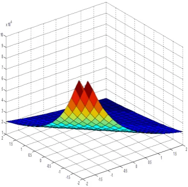
[image:10.595.210.403.546.738.2]

= 0. (83)

Figure 1. The M-error function forα= 0.5, β= 0.5, m= 8 of experiment 2

By implementing our method as presented in section 4, forn= 5,we obtain

u(x, y) = 1 +xy+(xy)

2

2 +

(xy)3

3 +

(xy)4

[image:11.595.196.385.54.247.2]

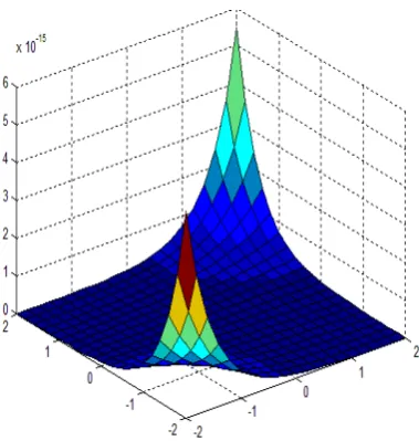
Figure 2. The M-error function forα= 0.5, β= 0.5, m= 15 of experiment 2

which is the first five terms of the two dimensional Taylor series ofe(xy).

We have observed that this method (the general shifted Jacobi matrix method) is very efficient for numerical approximation of the general high order linear PDEs with variable coefficients. Also, during the running of pro-grams, we found out the run time of the general shifted Jacobi matrix scheme is 2.015 second and the run time of the collocation method and Taylor approximation is 10.047 and 11.018 seconds, respectively. Thus in the case of the numerical solution of linear PDEs with variable coefficients, we prefer the general shifted Jacobi matrix scheme to the collocation method and Taylor approximation. This is the excellent advantage on the application of the general shifted Jacobi matrix scheme to the linear PDEs with variable coefficients. Also, closer look at the results of the general shifted Jacobi matrix scheme reveals that this method of solution is also stable.

7

Application of the method for the high order linear PDDEs

In this section, we report the numerical results obtained for a high order linear PDDE by the abovementioned procedure. This shows that it is straightforward to extend the method to the high order linear PDDEs as follows.

Experiment 3. Consider the fifth order linear PDDE [39] ∂5_u

∂x5 +x 2∂3u

∂y3 + 3x 5 ∂2u

∂x∂y + 12u= 720x+ 12y

4

+ 12x3, (85)

subject to the conditions

u(0, y) =y4_, ∂4_u

∂x4(0, y) +u(1, y)−u(−1, y) = 2, ∂3_u

∂x3(1, y) +y ∂u

∂x(0, y) = 126, ∂2u

∂x∂y(x,1/2)− ∂u

∂y(x,0) = 2x

2_{−4x, 3x}3∂u

∂y(x,1) + ∂u

∂x(x,−1) = 12x

3_{+ 3x}2_{+ 4x.} (86)

The exact solution of this equation is

u(x, y) =x6+y4−2x2y+x3. (87) By implementing the method as presented in section 4, form= 5 andm= 8 and also for different parameters ofαandβ, we obtain the approximate solutions. The Relative-error functions of this problem, are shown in figures 3 and 4. Also, tables 1 and 2 represent a comparison of the results of the present method with ref. [39].

Table 1. The Me.error for the method of [39] of experiment 3

n

m 4 5 6 7 8 9

6 3.38×10−12 _1.38×10−11 _1.55×10−11 _3.08×10−11 _5.53×10−10 _2.86×10−9

7 2.11×10−12 2.8×10−12 1.05×10−11 1.22×10−9 7.43×10−11 5.87×10−11 8 1.25×10−11 _9.66×10−12 _3.17×10−11 _4.14×10−11 _2.23×10−7 _1.12×10−8

[image:12.595.209.401.128.331.2]

Figure 3. The Relative-error function forα= 0.5, β= 0.5, m= 5, of experiment 3

[image:12.595.210.400.510.710.2]

Table 2. The Me.error for the present method forα= 0.4, β= 0.8 of experiment 3

n

m 4 5 6 7 8 9

6 2.46×10−12 _0.33×10−12 _3.77×10−12 _2.57×10−12 _3.89×10−11 _1.73×10−10

7 1.29×10−12 _1.18×10−13 _4.25×10−12 _0.17×10−9 _4.99×10−11 _3.39×10−12

8 1.09×10−11 _8.64×10−13 _1.61×10−12 _3.88×10−11 _1.22×10−7 _1.01×10−9

9 0.44×10−10 _7.39×10−12 _1.22×10−11 _7.17×10−11 _5.11×10−10 _1.32×10−8

8

Conclution

In this paper, we have introduced a new and efficient approach for numerical approximation of the second order linear PDDEs with variable coefficients. The method is based on the approximation of an exact solution with the two dimensional shifted Jacobi polynomial approximation with variable coefficients in the two dimensional Taylor series. Implementation of the method reduces the problem to a system of algebraic equations. Hence, the applicability of the present work is in considering of the general second order linear PDDE (1), whereas the other papers monitor only the particular cases of our general study. Also, using the general shifted Jacobi polynomials as the basis functions for numerical approximation wherein the shifted Chebyshev and Legendre polynomials are the particular cases of them, is the other superiority of the present study. Furthermore, the text experiments represent the accuracy and the efficiency of the method with only few terms in the expansion of Taylor series.

Acknowledgements

We are grateful to the reviewers and the editor for their helpful comments and suggestions which indeed improved the quality of this manuscript.

REFERENCES

[1] R. Agarwal, D. ORegan, Ordinary and Partial Differential Equations, Springer, 2009.

[2] L.C. Evans, Partial Differential Equations, American Mathematical Society, 1999.

[3] W.E. Schiesser, G.W. Griffiths, A compendium of partial differential equation models (method of Lines Analysis with Matlab), Cambridge University, 2009.

[4] J. Geiser, Decomposition methods for differential equations( Theory and Applications), Taylor and Francis, 2009.

[5] A.M. Wazwaz, Partial Differential Equations and Solitary Waves Theory, Springer, 2009.

[6] R. Camassa, D. Holm, An integrable shallow water equation with peaked solitons, Phys. Rev. Lett, vol. 71, pp. 1661-1664, 1993.

[7] A. Degasperis, M. Procesi, Asymptotic Integrability, Symmetry and Perturbation Theory, World Scientific, vol. 20, pp. 23-37, 1999.

[8] V. Eguiluz, E. Hernandez-Garcia and O. Piro, Boundary effects in the complex Ginzburg- Landau equation, Internat. J. Bifur. Chaos, vol. 23, pp. 2209-2214, 1999.

[9] B. Fuchssteiner, Some tricks from the symmetry-toolbox for nonlinear equations: Generalization of the Camassa-Holm equation, Physica D, vol. 95, pp. 229-243, 1996.

[10] B. Fuchssteiner and A. Fokas, Sympletic structures, their Backlund transformations and hereditary symmetries, Physica D, vol. 4 , pp. 47-66, 1981.

[11] Malfliet W., Solitary wave solutions of nonlinear wave equations, Am. J. Phys, vol. 60, pp. 650- 654, 1992.

[12] H. Holden, K.H. Karlsen, K.A. Lie, N.H. Risebro, Splitting methods for partial differential equations with Rough Solutions (Analysis and MATLAB programs), European Mathematical Society, 2010.

[13] K. W. Morton, D. F. Mayers, Numerical solution of partial differential equations, Cambridge University, 2009.

[14] M.H. Giga, Y. Giga, J. Saal, Nonlinear partial differential equations (Asymptotic Behavior of Solutions and Self-Similar Solutions), Springer, 2010.

[16] P. Solin, Partial differential equations and the finite element method, John wiley and sons, 2008.

[17] Cenk Kesan, Chebyshev polynomial solutions of second-order linear partial differential equations, Appl Math Comput, vol. 134, pp. 109-124, 2003.

[18] C. Kesan, Taylor polynomial solutions of second order linear partial differential equations, Appl Math Comput, vol. 152, pp. 29-41, 2004.

[19] A.M. Wazwaz, A comparison between the variational iteration method and Adomian decomposition method,Comput Appl Math, vol. 207, pp. 129-136, 2007.

[20] A.M. Wazwaz, S.M. Sayed, A new modification of Adomian decomposition method for linear and nonlinear operators. Appl Math Comput, vol. 122, pp. 393-405, 2011.

[21] S.H. Ho, C.K. Chen, Analysis of general elastically end restrained non-uniform beams using differential transform, Appl Math Model, vol. 22, pp. 219-234, 1998.

[22] N. Bildik, A. Konuralp, F.O. Bek, S. Kucukarslan, Solution of different type of the partial differential equation by differential transform method and Adomian’s decomposition method, Appl Math Comput, vol. 172, pp. 551-567, 2006.

[23] Z.M. Odibat, C. Bertelle, M.A. Alaoui, G.H.E. Duchamp, A multi-step differential transform method and application tonon-chaotic or chaotic systems, Comput Math Appl, vol. 59, pp. 1462-1472, 2010.

[24] W. G. Szymczak, I. Babuska, Adaptivity and error estimation for the finite element method applied to convection diffusion problems, SIAM J. Number. Anal, Vol. 21, No. 5, 1984.

[25] I. Babuska, J. E. Osborn, Generalized Finite Element Methods: Their Performance and Their Relation to Mixed Methods, SIAM J. Number. Anal, vol. 20, No. 3, 1983.

[26] I. Babuska, The Finite Element Method with Penalty, Mathematics of Computation, vol. 27, No. 122, 1973.

[27] I. Babuska, The Finite Element Method for Infinite Domains, Mathematics of Computation, vol. 26, No. 117, 1972.

[28] F. Shakeri, M. Dehghan, A finite volume spectral element method for solving magnetohydrodynamic (MHD) equations, Applied Numerical Mathematics, vol. 61, pp. 1-23, 2011.

[29] A. Ahmadian, M. Suleiman, S. Salahshour and D. Baleanu, A Jacobi operational matrix for solving a fuzzy linear fractional differential equation, Advances in Difference Equations, vol. 34, pp. 104-120, 2013.

[30] B. Y. Guo, J. Shen, L. L. Wang, Generalized Jacobi polynomials/functions and their applications, Applied Numerical Mathematics, vol. 59, pp. 1011-1028, 2009.

[31] D. Funaro, Polynomial Approximations of Differential Equations. Springer-Verlag, 1992.

[32] J.S. Hesthaven, S. Gottlieb, D. Gottlieb, Spectral Methods for Time-Dependent Problems, first ed, Cambridge Univer-sity, 2007.

[33] A. Imani, A. Aminataei, A. Imani, Collocation method via Jacobi polynomials for solving nonlinear ordinary differential equations, Int. J. Math. Math. Sci., Article ID 673085, 11P, 2011.

[34] M. R. Eslahchi, M. Dehghan, Application of Taylor series in obtaining orthogonal operational matrix, J. Comput. Math. Appl, vol. 61, pp. 2596-2604, 2011.

[35] M.R. Eslahchi, M. Dehghan, S. Ahmadi-Asl, The general Jacobi matrix method for solving some nonlinear ordinary differential equations, Appl. Math. Model, vol. 36, pp. 3387-3398, 2012.

[36] M. Razzaghi, S. Yousefi, Legendre wavelets method for the nonlinear Volterra- Fredholm integral equations, Math. Comput. Simul, vol. 70, pp. 1-8, 2005.

[37] S.A. Yousefi, M. Behroozifar, Operational matrices of Bernstein polynomials and their applications, Inter Systems Scie, vol. 32, pp. 709-716, 2010.

[38] H. Danfu, S. Xufeng, Numerical solution of integro-differential equations by using CAS wavelet operational matrix of integratio, Appl Math Comput, vol. 194, pp. 460-466, 2007.