R E S E A R C H
Open Access
Nested multiple imputation in large-scale
assessments
Sebastian Weirich
1*, Nicole Haag
1, Martin Hecht
1, Katrin Böhme
1, Thilo Siegle
1and Oliver Lüdtke
2* Correspondence:
1Institute for Educational Quality
Improvement, Humboldt-Universität zu Berlin, Unter den Linden 6, 10099 Berlin, Germany Full list of author information is available at the end of the article
Abstract
Background:In order to measure the proficiency of person populations in various domains, large-scale assessments often use marginal maximum likelihood IRT models where person proficiency is modelled as a random variable. Thus, the model does not provide proficiency estimates for any single person. A popular approach to derive these proficiency estimates is the multiple imputation of plausible values (PV) to enable subsequent analyses on complete data sets. The main drawback is that all variables that are to be analyzed later have to be included in the imputation model to allow the distribution of plausible values to be conditional on these variables. These background variables (e.g., sex, age) have to be fully observed which is highly unlikely in practice. In several current large-scale assessment programs missing observations on background variables are dummy coded, and subsequently, dummy codes are used additionally in the PV imputation model. However, this approach is only appropriate for small proportions of missing data. Otherwise the resulting population scores may be biased.
Methods:Alternatively, single imputation or multiple imputation methods can be used to account for missing values on background variables. With both imputation methods, the result is a two-step procedure in which the PV imputation is nested within the background variable imputation. In thesingle+multiple-imputation(SMI), each missing value on background variables is replaced by one value. Inthe multiple+multiple-imputation(MMI), each missing value is replaced by a set of imputed values. MMI is expected to outperform SMI as SMI ignores the uncertainty due to missing values in the background data.
Results:In a simulation study, both methods yielded unbiased population estimates under most conditions. Still, the recovery proportion was slightly higher for the MMI method.
Conclusions:The advantages of the MMI method are apparent for fairly high
proportions of missing values in combination with fairly high dependency between the latent trait and the probability of missing data on background variables.
Keywords:Large-scale assessment; Missing data; Imputation; Simulation; Item response theory
Background
Several large-scale assessment programs such as the National Assessment of Educa-tional Progress (NAEP), the Trends in InternaEduca-tional Mathematics and Science Study (TIMSS), and the Programme for International Student Assessment (PISA) employ item response theory (IRT) methods to measure the achievement of populations of ex-aminees in various domains, for example, reading and science, for the purpose of
system monitoring. The central interest is not to obtain individual proficiency scores but to obtain population and subpopulation estimates of person proficiency, denoted byθ. In addition to the item responses, the estimation process includes background in-formation for each person (often collected via questionnaires) comprising a multitude of variables, such as demographic, social, or motivational variables. Because these vari-ables may be associated with θ, they are of particular importance in the estimation of subpopulation differences. Large-scale assessment programs are often confronted with the problem of missing values in item responses or in background data. Planned miss-ing data in the item responses are a direct consequence of multiple matrix samplmiss-ing de-signs (Frey et al. 2009; Gonzalez & Rutkowski 2010). Methods of item and person parameter estimation which incorporate missing data in the item responses have long been developed and have been proved to be suitable (Lord 1974, 1983; Mislevy et al. 1992). By contrast, a considerable amount of missing data in background variables may lead to biased estimates of population parameters (Rutkowski 2011). Therefore, the present article examines the problem of missing data in background information when population estimates are of interest. We compared two methods that are based on im-putation methods with regard to the bias and root mean square error (RMSE) of popu-lation parameters. The results support the implementation of multiple imputation methods in the treatment of missing data in background information.
Item and person parameter estimation
In large-scale assessments, the estimation of item and person parameters commonly uses the marginal maximum likelihood (MML) method (Embretson & Reise 2000; Tuerlinckx et al. 2004; Wilson & De Boeck 2004). Conceptually, the estimation process is composed of two parts: theitem response model, which results from an analysis of the response pat-terns, and thepopulation model, which results from incorporating background informa-tion (Adams & Wu 2007). von Davier et al. (2009) refer to these two parts as the likelihood function and the prior distribution function. A model that comprises both parts is called aconditioning modelor combined model (Adams & Wu 2007).
In the item response model, the categorical response patterns to a set of test items are modeled as the dependent variable in a logistic regression with item difficulties and person proficiencies as independent variables. Adams and Wu (2007) and Adams et al. (1997) described the model in its generalized form. For the purpose of illustra-tion, we will use the special case of a unidimensional model with dichotomous items (Rasch model):
logitðP Xð ni¼1ÞÞ ¼θn−bi; ð1Þ
on background variables, the population model may be augmented to a regression model with several predictors (Adams & Wu 2007):
θn¼YnβþEn ð2Þ
whereYnis a vector ofufixed and known values for a set ofuvariables related to each person, andβis the corresponding vector of regression coefficients to be estimated.En is assumed to be independently and identically normally distributed with mean zero and varianceσ2; that is,En~N(0,σ2). The population model now incorporates fixed and random effects and provides a priori information about the expected person distribu-tion given all available background informadistribu-tion (von Davier et al. 2009).
The conditioning model is the item response model multiplied by the population model (Adams & Wu 2007; Embretson & Reise 2000). Hence, the conditioning model captures information from the test items (expressed in the item response model) and background information (expressed in the population model). Hence, it offers the opportunity to specify a population distribution of persons consisting of several sub-populations. This is especially important if the population distribution is conditional on several demographic variables rather than being a simple (unconditional) normal distribution.
Types of missing data and their effects on the estimation process
In large-scale assessments, three types of missing data can be distinguished. The first one is rather fundamental: IRT models are usually intended to measure proficiencies of persons. As each person’s individual proficiency θn is considered to be a latent con-struct, θ is an inherently unobserved (i.e., missing) variable. Missing data in the indi-vidual response pattern (the 0/1 answers of persons to test items) constitute the second type, and missing data in background information constitute the third type of missing data.
First type of missing data: inherently missingθ
values allows investigators to adequately quantify the uncertainty in the parameter estimation of subsequent analyses.
The imputation of plausible values can be conditioned on background information by including some demographic variables when specifying the population model. Similar to the recommendations made for multiple imputation (Rubin 1987), it is crucial to include all variables that may be used in subsequent analyses in order to ensure unbiased estimation of their effects on achievement (Mislevy et al. 1992; von Davier et al. 2009).
Second type of missing data: missing data in the item responses
The second (and also the third) type of missing data concerns missing values in data that are expected to be observed. However, the second type of missing data likewise is not a problem for parameter estimation, if some conditions are met. Missing data in the item responses are a direct consequence of multiple matrix sampling designs (Frey et al., 2009; Gonzalez & Rutkowski 2010). As large samples of items are used to com-prehensively cover the test constructs, only a subset of items is presented to each per-son to keep the individual workload within acceptable boundaries. Such missing responses which result from giving samples of items to samples of persons are often called missing by design(Enders 2010). If the test booklets are randomly distributed to the persons, these data are assumed to be missing completely at random (MCAR). MCAR means that missing values on a variable neither depend on values of other vari-ables in the model nor on values of the variable itself (Graham 2009; Rubin 1987). By contrast, responses that a person has chosen to omit are often treated as incorrect re-sponses. See Lord (1974, 1983) and Ludlow and O’leary (1999) for a discussion of this procedure.
Third type of missing data: missing data in background information
The third type of missing data—which is the focus of the present article—concerns missing values on background variables which are inherently due neither to the latent variable modeling of θnor to the test design. In the population model (Equation 2), it is assumed that background variables are measured without error becauseYnis a vector of fixed and known values (Adams & Wu 2007). In principle, the same problem applies when missing values occur in ordinary least squares regression models (e.g., Little 1992): The corresponding procedures require that all variables be fully observed.
Approaches to dealing with missing data in background information
Dummy coding
In several current large-scale assessment programs (Allen et al. 2001; Foy et al. 2008; OECD 2009) missing observations were dummy coded and the dummy variables were subsequently used in the population model. However, Schafer and Graham (2002) pointed out that this method merely redefines the parameters as the population model now contains two effects for a variableXin the population model: one effect for the re-spondents and another effect for the nonrere-spondents. Moreover, this approach does not take a possible missing at random (MAR) mechanism into account. MAR means that missing values on a certain variable may depend on values of other variables in the model but not on values of the variable itself. Allison (2002) demonstrated that even in the case of MCAR, dummy-variable adjustment may lead to biased estimates in ordinary least squares regression when the proportion of missing data is substantial (i.e., 50%).
Rutkowski (2011) carried out a simulation study to explore the impact of missing values on background variables on proficiency estimates when missing values on back-ground variables were dummy coded, focusing on the estimation of differences in group means. Under an MAR condition with a maximum of 20% of missing values, the differences in group means were estimated without bias. However, both group means were biased in the same direction. Rutkowski termed this atandem shift.Although this tandem shift preserved subgroup differences, it may lead to erroneous conclusions if the results are to be expressed on a predefined scale, for example, to estimate trend effects between different cohorts (Mazzeo & Von Davier 2008). Rutkowski (2011) pointed out that the estimation of subgroup differences can be problematic if the pro-portions of missing values on the background variables differ between groups. In sum-mary, dummy coding may be appropriate if it is combined with assessment strategies that minimize the proportion of missing values in background information. If this is not the case, defining dummy codes for missing observations may be questionable from a theoretical point of view (Schafer & Graham 2002) and may also lead to biased mean estimates (Rutkowski, 2011). Hence, alternative procedures have to be applied.
Single + Multiple Imputation (SMI)
Instead of using dummy codes, missing values on background data may be imputed prior to estimating the parameters of the conditioning model (OECD 2006; Weirich et al. 2012. In order to impute the missing data, we have to construct an imputation model which includes all variables that may be related to the occurence of missing data under an MAR assumption. Thus, the population model used to generate the plausible values includes imputed data on the background variables.
The SMI procedure contains a sequence of four steps. The first step is the specifica-tion of the item response model (often referred to as calibraspecifica-tion). As the aim is to esti-mate the item parameters only, a simple MML population model without background information can be chosen as θn=μ+En, withEn~N(0,σ2). The mean of the popula-tion distribupopula-tion is often defined to be zero, i.e., μ= 0. Hence, to calibrate items, miss-ing values in background variables can be ignored.
onθ, we should includeθinto the imputation model. However, individualθnvalues are estimated in a later step, therefore we have to use a proxy for θ, for example, the per-centage of correct responses or point estimates (e.g., MLEs or WLEs) for each person from the item response model. In this study, we will use the latter one.
The third step is the estimation of the conditioning model’s parameters. We jointly use the item responses and the (imputed) background information for estimation. In contrast to the item response model, θn=Ynβ+En. Yn does not contain any missing values because all missing values were imputed in the third step. All background vari-ables are treated as if they were fully observed. A common practice is to consider the item parameters obtained in the first step as the true item parameters (von Davier et al. 2007).
The fourth and last step is the imputation of plausible values. The imputation model for this step is the conditioning model. Hence, the process of handling different sources of missing data comprises two imputation procedures: a single imputation of back-ground variables and a multiple imputation of latent person estimates (θn). To avoid confusion between both, we henceforth refer to the first one (step 2) as the imputation model and to the second one (step 4) as the conditioning model. Both imputation steps are not independent because the imputed data from step 2 are used in step 4.
The SMI procedure should help to minimize bias in the population model when missing values on background variables depend on θ.However, there is an uncertainty in the prediction ofθin the population model due to missing values on background in-formation. The SMI procedure may not adequately represent this uncertainty because the population model treats observed and imputed values in the same way. For ex-ample, consider two groups with different proportions of missing values on background variables: The uncertainty in the group mean estimates should differ between the groups because we have more observed data in one group than in the other. However, this is not represented in the model if only a single imputation method is used for both groups. Although a bias in estimated group mean differences is unlikely, if the imput-ation model adequately captures the mechanism behind the missing data, the corre-sponding standard errors of the mean estimates may be underestimated (White et al. 2010), in particular if the rates of missing data in background variables are high.
Multiple + Multiple Imputation (MMI)
Nested imputation (Rubin 2003) or two-stage multiple imputation (Harel 2007; Harel & Schafer 2003; Reiter & Drechsler 2007; Reiter & Raghunathan 2007) explicitly man-ages two multiple imputation procedures in a dependent structure. The basic principle is described by Rubin (2003):
A few imputations of the first part are created (sayM), and then for each of these, several imputations of the second part are created (sayN). The standard combining rules for multiple imputation (the repeated imputation rules) have to be modified because the imputations within a nest are correlated, since they share a common set of imputed values for the first set of missing values. (p. 6)
assessments, this may be of particular interest as we may assume different mechanisms in order to account for missing values on θ and missing values on background vari-ables. Furthermore, MMI is preferable to SMI because MMI captures both sources of uncertainty: the uncertainty due to missing values on the background variables and the uncertainty due to the inherently missingθvalues.
To implement this method in a large-scale assessment context, we would have to ex-tend the SMI procedure described in the previous section. In the second step, we now create more than one imputation of the background data (which would result in, say, M= 5 data sets). Step 3 therefore has to be repeatedM times, once for each of theM imputed data sets. In step 4, we would draw Nplausible values from each of theM fit-ted conditioning models, which will result inM×Nplausible values overall. We would then apply the modified combining rules by Rubin (2003) to pool statistics based on these plausible values. A more detailed illustration of how the following combining rules are applied to the sets of plausible values is provided in Additional file 1.
LetQbe the quantity of interest (i.e., our set of plausible values). Q^ðm;nÞ is the mean
estimate of thenth plausible value in themth nest. The overall average Q, then, is:
Q¼ 1
MN
XM
m¼1
XN
n¼1
^
Qðm;nÞ: ð3Þ
Qm is a vector ofMmean estimates across theNplausible values in each nest
Qm¼ 1
N
XN
n¼1
^
Qðm;nÞ; ð4Þ
andU is the overall average of the associated variance estimates,
U ¼ 1
MN
XM
m¼1
XN
n¼1
Uðm;nÞ: ð5Þ
LetMS(b)be the between-nest mean square,
MSð Þb ¼ N M−1
XM
m¼1
Qm−Q
ð Þ2; ð
6Þ
and letMS(ω)be the within-nest mean square,
MSð Þω ¼ 1 M Nð −1Þ
XM
m¼1
XN
n¼1
Qðm;nÞ−Qm
2
: ð7Þ
The quantity
T ¼U þ 1
N 1þ
1
M
MSð Þb þ 1−1
N
MSð Þω ð8Þ
estimates the total variance of Q−Qð Þ. Estimation of the significance levels of Q are based on a Student-treference distribution,T−0:5ðQ−QÞ
etv. The degrees of freedom,v,
v−1¼ N
−11þM−1MSð Þb
T
!2
1
M−1þ
1−N−1
MSð Þω T
!2
1
M Nð −1Þ: ð9Þ
This procedure is computationally more extensive than the commonly applied dummy coding procedure and, to our knowledge, has not been used in any large-scale assessment program yet. However, from a theoretical point of view, MMI strategies seem especially appropriate as they explicitly account for several types of missing data in a dependent structure, which is common in large-scale assessments. The present art-icle therefore assesses whether using MMI leads to more precise estimates of the un-certainty of person parameters than SMI when the proportion of missing values on background variables is substantial. This question is of particular interest if it seems plausible that missing background data are MAR instead of MCAR. The study only in-vestigates the third type of missing data and assumes that missing values in the item re-sponses are MCAR (as a consequence of multiple matrix sampling) and missing values on background variables are MAR. Specifically, our study addressed the following re-search questions:
1. Does either SMI or MMI of missing values on background variables lead to unbiased estimates of subpopulation proficiency means, the mean subpopulation proficiency difference, and regression coefficients of proficiency on background variables?
2. Does either SMI or MMI of missing values on background variables lead to
unbiased estimates of standard errors of subpopulation proficiency means, the mean subpopulation proficiency difference, and regression coefficients?
We expected that both methods would lead to unbiased mean estimates and regres-sion coefficients. Moreover, the MMI method was expected to capture the uncertainty more adequately and was expected to result in slightly higher standard errors and slightly larger confidence intervals for parameters.
Method
We conducted a simulation study to compare the SMI and the MMI methods when missing proportions on background variables were substantial. Missing values on back-ground variables were assumed to be dependent on θ (i.e., an MAR condition was as-sumed for the simulation).
Simulation design
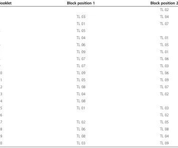
incomplete block design (see e.g., Frey et al. 2009; Gonzalez & Rutkowski 2010). The booklet design is displayed in Table 1. The original item difficulties from the LV 2011 were used to simulate the item responses. The item difficulties ranged from−2.995 to 2.689, which corresponds to a probability for a correct response ranging from 92.9 per-cent to 9.1 perper-cent. Item responses of N= 2,000 persons were simulated resulting in 400 valid responses per item.
Two uncorrelated background variables were used in the simulation. The first one, X1, was uniformly distributed with two levels 0 and 1 (i.e., a grouping variable splitting
the population into two subpopulations). The second one,X2, was normally distributed.
The true person proficiency distribution was simulated to depend on both background variables. The population model (see Equation 2) was
θn¼β1X1þβ2X2þEn; ð10Þ
with EneN 0;σ2θ
andσ2θ¼1:44. Equation 10 is used to both generate and analyze the data. In order to differentiate between the parameters of these models, we use asterisks for the parametersβ1 andβ2of the simulation model to indicate that these are true pa-rameters. In contrast, the parameters of the population model used to analyze the data are denotedβ1andβ2. Forβ1 andβ2, a combination of values of 0.1 and 0.4 were used,
which resulted in 2 × 2 = 4 conditions for the population model. The coefficients were chosen to mimic conditions which can be expected in real large-scale assessments. In
Table 1 Rotated block design to form test booklets
Booklet Block position 1 Block position 2
1 TL 02
2 TL 03 TL 04
3 TL 01 TL 07
4 TL 05
5 TL 04 TL 01
6 TL 06 TL 05
7 TL 09 TL 01
8 TL 07 TL 06
9 TL 07 TL 03
10 TL 09 TL 06
11 TL 05 TL 09
12 TL 08 TL 07
13 TL 04 TL 02
14 TL 08
15 TL 01 TL 03
16 TL 02
17 TL 02 TL 05
18 TL 06 TL 08
19 TL 08 TL 04
20 TL 03 TL 09
Note.TL = testlet. Empty cells mean that the corresponding position in the booklet is non-occupied. For example, booklet 1 only contains testlet 2.
the German National Assessment Study in secondary schools 2012, for example, the largest effect of socioeconomic status (SES) on proficiency is 49 points on the PISA scale with M= 500 and SD= 100 (Kuhl et al. 2013). This corresponds to a regression coefficient of about .45. For each background variable, 25% and 40% of the values were deleted, mimicking empirical findings on proportions of missing data for sensitive vari-ables (i.e. SES) when the completion of questionnaires is voluntary (Stanat et al. 2012). The patterns of missing data of the background variables were in turn created to be dependent on true person proficiencies. For each background variable, the polyserial correlation of the missing pattern with the true person proficiencies was −.10 or −.40. To keep the number of simulations manageable, we refrained from testing against a baseline condition (i.e., 0% missing values or a zero correlation) as we did not expect to find any bias under these conditions.
The simulation was set up using a full-factorial experimental design so that all pos-sible combinations would be represented. We varied the following factors and factor levels:
– Regression coefficients in the population model:β1={.1,.4} andβ2={.1,.4}
– Proportions of missing data for both background variablesX1andX2:m(X1) =
{.25,.4} andm(X2) = {.25,.4}
– Correlations between the patterns of missing data in both background variables and
θ*
:d(X1,θ*) = {−.1,−.4} andd(X2,θ*) = {−.1,−.4}
In the next step, the 20 booklets were randomly distributed to virtual persons. Using the true person proficiency scores from Equation 10 and the known item parameters, the response probability for personn and itemiwas defined according to the item re-sponse model (see Equation 1):
P Xð ni¼1Þ ¼
eθn−bi
1þeθn−bi: ð11Þ
Each response Xni was generated by sampling a value from a uniform distribution across the interval [0, 1]. If the sampled value was between 0 andP(Xni= 1),Xniwas set to 1. Otherwise,Xniwas set to 0.
We used the package TAM (Kiefer et al. 2013) in R (R Core Team 2014) to specify a marginal IRT model without conditioning on background variables, where the item pa-rameters were fixed at their known values. This analysis was done for the sole purpose of obtaining a WLE for each person. The WLE served as a rough point estimate of the unknown true proficiency score.
Next, the missing values of both background variables were imputed using the R package MICE (van Buuren & Groothuis-Oudshoorn 2011). The imputation model consisted of three variables—X1, X2,and the WLE—in a fully conditional specification
(see van Buuren 2007) to account for the process that created the missing data. Two different imputation methods were applied. ForX1, we used a logistic regression
imput-ation according to its binomial distribution. ForX2, we used predictive mean matching.
SMI method
The first imputed data set was used to specify the population model in order to estimate the posterior distribution of the person parameters with item parameters fixed at their known values. Using TAM, twenty plausible values were drawn from the posterior distribution. The mean proficiency estimates were pooled across these 20 imputed values according to Rubin (1987). The regression estimates were taken from the latent regression part of the population model. Therefore, pooling was not necessary.
MMI method
The method described above was repeated M= 5 times, which resulted in 5 × 20 = 100 plausible values. The mean proficiency estimates were pooled over 100 imputed values according to Rubin (2003), whereas the regression estimates were pooled over M= 5 imputed values according to Rubin (1987).
Measures
The estimates of interest were
– the mean proficiency estimates in both subpopulations (i.e.,θX1¼0andθX1¼1)
– the mean proficiency difference (i.e.,θX1¼1−θX1¼0)
– the estimated coefficientβ2in the latent regression model
The analyses were repeated 1,000 times for each of the 64 conditions. For all esti-mates mentioned above, three measures were of particular interest in each condition. To examine whether a bias in the corresponding estimates occurred, we computed
Bias xð Þ ¼N−1X
N
i¼1 xi−x
ð Þ; ð12Þ
whereNis the number of replications,xiis the estimate in theith replication, and xis the true parameter which was used for data generation. For example, if we consider the bias in the regression coefficientβ2,xiis the estimate ofβ2in theith replication, andx
=β2. If we consider the bias in the subpopulation differences, xi is the estimate of
θX1¼1−θX1¼0in theith replication, andxis the true subpopulation difference, i.e.x=β
1. The root mean square error (RMSE) between the true xand the estimatedxi parame-ters were computed by using
RMSE xð Þ ¼
ffiffiffiffiffiffiffiffiffiffiffiffiffiffiffiffiffiffiffiffiffiffiffiffiffiffiffiffiffiffi
N−1X
N
i¼1 xi−x
ð Þ2
v u u
t : ð13Þ
confidence interval would include the true value in 95% of all cases. The 95% confi-dence interval forxiwas computed as
CI95ð Þ ¼xi xi1:96⋅SE xð Þi : ð14Þ
To identify whether the bias or the RMSE depended on the simulated conditions, we calculated ANOVA effect sizes across all replications of the simulation. All ANOVA analyses contained the following seven factors, each with two levels: β1, β2, missing proportion on X1(m(X1)), missing proportion onX2(m(X2)), dependency betweenθ*
and the missing values onX1(d(X1,θ*)), dependency betweenθ*and the missing values
onX2(d(X2,θ*)), and the imputation method (SMI vs. MMI). For the sake of
concise-ness and clarity of results, we only computed main effects, two-way interactions, and
three-way interactions in a common model. Hence, 7þ 7 2 þ
7
3 ¼63 effects were estimated. For the same reason, only effects for which the effect sizeη2exceeded 0.005 are displayed. Moreover, we computed ANOVAs without interaction effects in order to describe whether the addition of interaction effects leads to an increase in ex-plained variance.
To identify whether the recovery proportion depended on the simulated conditions, we conducted a logistic regression analysis. For each of the 1,000 replications of the 64 simulated conditions, we created a dummy code that equaled 1 if the confidence inter-val of the corresponding estimate incorporated the true inter-value and 0 otherwise. This dummy code was used as the dependent variable in a logistic regression analysis. All re-gression analyses contain the seven factors mentioned above, each with two levels.
Results
The following section summarizes the results of the simulation, focusing on differences between the SMI and the MMI methods. First, we present the bias for the three esti-mates’mean proficiency difference,β1and β2. We examine whether the bias was
influ-enced by conditions of the simulation using descriptive analyses and ANOVA effect size estimation. The same procedure was carried out for the RMSE and the recovery proportion.
The table for the means of all measures in all of the 64 conditions for both single and nested imputation of background variables is provided in Additional file 1 (Table B1).
Bias
Tables 2 and 3 display ANOVA effect size estimates of bias in the subpopulation differ-ences (Table 2) and of bias in the regression coefficient β2 (Table 3). Across all
simulated conditions, the bias for all estimates was negligible (mean bias in the subpop-ulation differences =−0.016; mean bias for regression coefficient β2= 0.017). Moreover,
the differences between SMI and MMI were negligible (the main effect of imputation method failed to account for a substantial amount of variance in the bias of the sub-population differences and the regression coefficient β2). Whereas the overall bias was
small, some conditions were associated with higher bias: For example, higher correla-tions between the patterns of missing data inX1andθ*caused a higher bias in the
differences and in the estimation of β2. Higher proportions of missing data for
back-ground variableX1caused a bias in the estimation ofβ2. However, most ANOVA effect
sizes were small. For example, the seven main effects of the ANOVA analysis displayed in Table 2 together only account for 7.3% of the explained variance, whereas all 64 ef-fects together account for 33.2% of the explained variance. Considering Table 3, the seven main effects only account for 5.7% of the explained variance, whereas all 64 effects account for 20.4% of the explained variance. The bias was therefore rarely asso-ciated with a single factor (e.g., a large proportion of missing values alone) but rather with combinations of (adverse) conditions (e.g., a large proportion of missing values and a high level of dependence of the pattern of missing data on true person Table 2 ANOVA effect size table for bias in subpopulation
Differencesfactor SS η2
d(X1,θ*) ×d(X2,θ*) 52.14 0.062
d(X1,θ*) 45.18 0.054
β
1m Xð Þ1 21.48 0.025
β
2d Xð 1;θÞ 19.98 0.024
β
1m Xð Þ 1 d Xð 2;θÞ 17.65 0.021
m(X1) ×m(X2) 13.54 0.016
β
2d Xð 1;θÞ d Xð 2;θÞ 10.87 0.013
β
2m Xð Þ 1 d Xð 1;θÞ 7.24 0.009
β
2m Xð Þ2 7.13 0.008
β
2m Xð Þ 2 d Xð 2;θÞ 6.96 0.008
β
1β2d Xð 1;θÞ 6.08 0.007
β
1β2 5.62 0.007
m(X1) ×m(X2) ×d(X2,θ*) 4.81 0.006
m(X1) ×d(X2,θ*) 4.66 0.006
d(X2,θ*) 4.56 0.005
β
2m Xð Þ 1 d Xð 2;θÞ 4.47 0.005
m(X1) ×d(X1,θ*) ×m(X2) 4.40 0.005
Residuals 563.55
Total 844.02
Table 3 ANOVA effect size table for bias in regression coefficientβ2
Factor SS η2
m(X1) 12.90 0.087
β
1β2 4.13 0.028
d(X2,θ*) 3.17 0.022
β
1m Xð Þ1 2.42 0.016
β
1 2.40 0.016
β
1β2d Xð 1;θÞ 1.36 0.009
β
1d Xð 2;θÞ 1.19 0.008
β
1β2m Xð Þ2 1.04 0.007
β
2m Xð Þ 2 d Xð 2;θÞ 0.82 0.006
Residuals 110.01
proficiencies). Both SMI and MMI are therefore able to compensate for a single ad-verse condition. As expected, the imputation method (SMI vs. MMI) did not affect the bias—all ANOVA analyses revealed only negligible main effects of the simulation methods or interaction effects of the simulation method and the other factors.
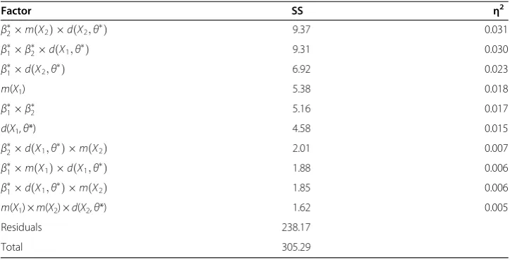
RMSE
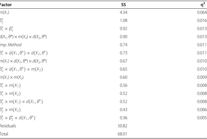
Tables 4 and 5 display ANOVA effect size estimates for the RMSE in the subpopulation differences (Table 4) and in the regression coefficient β2(Table 5). Across all simulated
conditions, the RMSE for the subpopulation differences was .076. The mean RMSE for the regression coefficientβ2was .035. The RMSE differed between the two imputation
methods, but only slightly and only for the regression coefficient β2: The RMSE was
.037 for the single imputation method and .032 for the nested imputation method. This main effect was significant (η2= 0.011, see Table 5). Considering Table 4, the seven main effects of the ANOVA analysis only account for 4.4% of the explained variance, whereas all 64 effects account for 22% of the explained variance. Considering Table 5, the main effects account for 10% of the explained variance, whereas all 64 effects ac-count for 25.3% of the explained variance.
Although we found a significant main effect of imputation method on the RMSE for the regression coefficientβ2, its effect size was small and the reduction of .037–.032 = .005 in
the RMSE is negligible.
Recovery proportion
We conducted logistic regression analyses to predict the probability that the confidence interval of an estimate (e.g.,β2) would include the true value. Tables B2 and B3 are
pro-vided in Additional file 1 and display the results of the logistic regression analyses for the recovery proportion of the subpopulation differences (Table B2) and regression co-efficientβ2(Table B3). Comparing the SMI and MMI methods, we found mean
recov-ery proportions of .83 versus .95 for the subpopulation differences, and .85 versus .96 for the regression coefficientβ2. The main effect for the imputation method was
signifi-cant both for subpopulation differences and for the regression coefficient β2. MMI
Table 4 ANOVA effect size table for the RMSE of subpopulation differences
Factor SS η2
β
2m Xð Þ 2 d Xð 2;θÞ 9.37 0.031
β
1β2d Xð 1;θÞ 9.31 0.030
β
1d Xð 2;θÞ 6.92 0.023
m(X1) 5.38 0.018
β
1β2 5.16 0.017
d(X1,θ*) 4.58 0.015
β
2d Xð 1;θÞ m Xð Þ2 2.01 0.007
β
1m Xð Þ 1 d Xð 1;θÞ 1.88 0.006
β
1d Xð 1;θÞ m Xð Þ2 1.85 0.006
m(X1) ×m(X2) ×d(X2,θ*) 1.62 0.005
Residuals 238.17
overall leads to a higher recovery proportion than SMI. Moreover, the advantage of MMI over SMI is particularly apparent in some specific conditions, for example, if the missing proportion on X1is 40% instead of 10% (line 23 in Table B2). This indicates
that the MMI method yields a higher recovery proportion if the proportion of missing values is large, or if the correlation between the patterns of missing data inX2andθ*is -.4
instead of -.1. To summarize, MMI seems appropriate for (a combination of ) some ad-verse conditions. This finding reflects the fact that the uncertainty in the imputed values, which results from some adverse conditions, is only incorporated in the MMI method.
Discussion
The goal of the present study was to compare two imputation methods—SMI and MMI—for handling missing data in background variables in large-scale assessment pro-grams. The first key question of the present paper was whether these imputation methods would allow unbiased estimation of subpopulation differences and coefficients in the latent regression model. The second question was related to the standard errors of the estimates: How often does the confidence interval include the true value?
Concerning the first research question of unbiased population estimates, none of the simulated conditions showed differences between SMI and MMI. The mean bias was negligible for both imputation methods. Some adverse factors (and especially combina-tions of adverse factors, e.g., a large proportion of missing values and a high level of de-pendence of the missing data pattern on true person proficiency) led to biases in the range of −0.145 to 0.092 for the subpopulation differences and −0.041 to 0.061 for the regression coefficientβ2.
Concerning the second research question, when considering the RMSE and especially the recovery proportion, the MMI method outperformed the SMI method. As the MMI method takes the between-imputation variance in the imputed background data Table 5 ANOVA effect size table for the RMSE of regression coefficientβ2
Factor SS η2
m(X1) 4.34 0.064
β
2 1.08 0.016
β
1β2 0.92 0.013
d(X1,θ*) ×m(X2) ×d(X2,θ*) 0.90 0.013
imp. Method 0.74 0.011
β
1d Xð 1;θÞ d Xð 2;θÞ 0.73 0.011
m(X1) ×d(X1,θ*) ×d(X2,θ*) 0.67 0.010
β
2d Xð 1;θÞ m Xð Þ2 0.65 0.010
m(X1) ×m(X2) 0.60 0.009
β
1m Xð Þ1 0.56 0.008
β
1m Xð Þ2 0.52 0.008
β
2m Xð Þ 1 d Xð 1;θÞ 0.52 0.008
β
2m Xð Þ2 0.43 0.006
β
1β2d Xð 1;θÞ 0.36 0.005
Residuals 50.82
into account, the standard errors of the regression coefficient β2and of the
subpopula-tion difference accurately reflected the uncertainty due to the amount of missing data. The estimates of the regression coefficient β2varied less between the replications and
resulted in lower RMSEs. The differences between the two imputation methods, how-ever, were apparent only for substantial proportions of missing data of about 40%, which may occur empirically for some sensitive variables such as SES (Stanat et al. 2012). Hence, we recommend using MMI instead of SMI if the missing data proportion is substantial andif researchers are interested not only in unbiased estimates (e.g., for purely descriptive purposes) but also in unbiased standard errors of these estimates (e.g., for significance testing).
In general, we conclude that imputation methods can provide a suitable alternative to dummy coding, which is flawed by some conceptual problems and may cause biased mean proficiency estimates if the proportion of missing values on the background vari-ables is substantial (Rutkowski 2011). To date, multiple imputation methods per se are widely established in large-scale assessments to estimate θn values, which are consid-ered to be inherently missing in the IRT framework, whereas the problem of missing data in background variables has rarely been tackled by imputation methods. Our ana-lyses show that MMI yields only small practical advantages compared to SMI at the cost of higher computational effort. Therefore, SMI should be a sufficient method in most applications.
Typically, large-scale assessments comprise a multitude of background variables, which are reduced to several uncorrelated principal components prior to the estimation of the population model. Compared to this procedure, the present simulation is highly simplified. In empirical applications where background variables typically are corre-lated, it is plausible to assume that the more background variables are included, the less problematic is a high proportion of missing values on a single variable as other vari-ables might compensate the loss of information. SMI and MMI methods may easily be combined with principal component analyses, which can be applied after the imput-ation of missing values in background variables. With MMI, this would result in several data sets, where the number of principal components may vary between the data sets.
experimental design (e.g., sample size, number of items, number of background vari-ables, or proportion of missing values on background variables). A further improve-ment of the imputation approach might be to include the unreliability of the WLE as a possible source of uncertainty into the imputation model. However, as a three-level nested imputation this would result in much more computational effort which may not be desirable in empirical applications.
Conclusion
The present study showed that nested imputation methods are suitable approaches to deal with missing values in both continuous and categorical background variables. Both SMI and MMI yield virtually unbiased estimates of subpopulation differences and re-gression coefficients for background variables with missing data. Concerning the esti-mation of standard errors, MMI more accurately reflect the uncertainty due to missing data in the background variables than SMI, resulting in slightly larger standard errors. However, the differences between imputation methods are small in non-extreme condi-tions of missing data. Thus, both SMI and MMI can be used to impute missing values on background variables in large-scale assessments to avoid the conceptual flaws and the possible biases associated with the common approach of dummy coding missing observations.
Additional file
Additional file 1:Appendix to the paper: Nested Multiple Imputation in Large-Scale Assessments.
Competing interests
The authors declare that they have no competing interests.
Authors’contributions
SW, NH and MH reviewed the literature. SW, NH, OL and TS designed the analysis. SW conducted the analysis and evaluated the results. SW wrote the manuscript. KB and OL read and revised the manuscript. TS and MH verified the simulation program code. All authors read and approved the final manuscript.
Acknowledgments
This work was supported by the Institute for Educational Quality Improvement at Humboldt-Universität zu Berlin, Berlin, Germany. The authors would like to thank two anonymous reviewers for their constructive help and support with improving this article.
Author details
1
Institute for Educational Quality Improvement, Humboldt-Universität zu Berlin, Unter den Linden 6, 10099 Berlin, Germany.2Leibniz Institute for Science and Mathematics Education (IPN), Centre for International Student Assessment,
Olshausenstraße 62, 24118 Kiel, Germany.
Received: 31 January 2014 Accepted: 1 October 2014
References
Adams, RJ, Wilson, M, & Wang, W-C. (1997). The multidimensional random coefficients multinomial logit model.Applied Psychological Measurement, 21(1), 1–23.
Adams, RJ, & Wu, ML. (2007). The Mixed-Coefficients Multinomial Logit Model: A Generalized Form of the Rasch Model. In M Von Davier & CH Carstensen (Eds.),Multivariate and Mixture Distribution Rasch Models(pp. 57–75). New York: Springer.
Allen, NL, Donoghue, JR, & Schoeps, TL. (2001).The NAEP 1998 Technical Report. Washington: National Center for Educational Statistics.
Allison, PD. (2002).Missing Data. Thousand Oaks, CA: Sage Publications.
Bock, RD, & Aitkin, M. (1981). Marginal maximum likelihood estimation of item parameters: application of an EM algorithm.Psychometrika, 46(4), 443–459.
De Boeck, P. (2008). Random item IRT models.Psychometrika, 73(4), 533–559. doi: 10.1007/s11336-008-9092-x. Embretson, SE, & Reise, SP. (2000).Item Response Theory for Psychologists. Mahwah, NJ: Erlbaum.
Foy, P, Galia, J, & Li, I. (2008). Scaling the Data from the TIMSS 2007 Mathematics and Science Asssessment. In JF Olson, MO Martin, & IVS Mullis (Eds.),TIMSS 2007 Technical Report(pp. 225–280). Chestnut Hill, MA: TIMSS & PIRLS International Study Center, Lynch School of Education, Boston College.
Frey, A, Hartig, J, & Rupp, AA. (2009). An NCME instructional module on booklet designs in large-scale assessments of student achievement: theory and practice.Educational Measurement: Issues and Practice, 28(3), 39–53.
Gonzalez, E, & Rutkowski, L. (2010). Principles of multiple matrix booklet designs and parameter recovery in large-scale assessments.IEA-ETS Research Institute Monograph, 3, 125–156.
Graham, JW. (2009). Missing data analysis: making it work in the real world.Annual Review of Psychology, 60, 549–576. Harel, O. (2007). Inferences on missing information under multiple imputation and two-stage multiple imputation.
Statistical Methodology, 4, 75–89.
Harel, O, & Schafer, JL. (2003).Multiple Imputation in two Stages. Washington DC: Paper presented at the Proceedings of Federal Committee on Statistical Methodology Research Conference.
Kiefer, T, Robitzsch, A, & Wu, M. (2013). TAM: test analysis modules (R package version 0.5-21). Retrieved from http://CRAN.R-project.org/package=TAM.
Kuhl, P, Siegle, T, & Lenski, AE. (2013). Soziale Disparitäten [Social disparities]. In HA Pant, P Stanat, U Schroeders, A Roppelt, T Siegle, & C Pöhlmann (Eds.),IQB-Ländervergleich 2012. Mathematische und naturwissenschaftliche Kompetenzen am Ende der Sekundarstufe I[The IQB National Assessment study 2012—Competencies in mathematics and the sciences at the end of secondary level] (S. 275–296). Münster: Waxmann.
Little, RJA. (1992). Regression with missing X’s: A review.Journal of the American Statistical Association, 87(420), 1227–1237. Lord, FM. (1974). Estimation of latent ability and item parameters when there are omitted responses.Psychometrika, 39
(2), 247–264.
Lord, FM. (1983). maximum likelihood estimation of item response parameters when some responses are omitted. Psychometrika, 48(3), 477–482.
Ludlow, LH, & O’leary, M. (1999). Scoring omitted and not-reached items: practical data analysis implications.Educational and Psychological Measurement, 59, 615–630. doi:10.1177/0013164499594004.
Mazzeo, J, & Von Davier, M. (2008).Review of the Programme for International Student Assessment (PISA) Test Design: Recommendations for Fostering Stability in Assessment Results. Available at: doc.ref. EDU/PISA/GB(2008)28. Mislevy, RJ, Beaton, AE, Kaplan, B, & Sheehan, KM. (1992). Estimating population characteristics from sparse matrix
samples of item responses.Journal of Educational Measurement, 29, 133–161.
OECD. (2006).Assessing Scientific, Reading and Mathematical Literacy. A Framework for PISA 2006. Paris: OECD. OECD. (2009).PISA 2006 Technical Report. Paris: OECD.
R Core Team. (2014).R: A Language and Environment for Statistical Computing. (Version 3.1.0). Vienna, Austria: R Foundation for Statistical Computing. Retrieved from http://www.R-project.org/.
Reiter, JP, & Drechsler, J. (2007). Releasing multiply-imputed synthetic data generated in two stages to protect confidentiality.IAB Discussion Paper, 2007(20)1–18.
Reiter, JP, & Raghunathan, TE. (2007). The multiple adaptions of multiple imputation.Journal of the American Statistical Association, 102, 1462–1471.
Rubin, DB. (1987).Multiple Imputation for Nonresponse in Surveys. New York: Wiley.
Rubin, DB. (2003). Nested multiple imputation of NMES via partially incompatible MCMC.Statistica Neerlandica, 57(1), 3–18.
Rutkowski, L. (2011). The impact of missing background data on subpopulation estimation.Journal of Educational Measurement, 48(3), 293–312.
Schafer, JL, & Graham, JW. (2002). Missing data: our view of the state of the art.Psychological Methods, 7, 147–177. Stanat, P, Pant, HA, Böhme, K, & Richter, D (Eds.). (2012).Kompetenzen von Schülerinnen und Schülern am Ende der
vierten Jahrgangsstufe in den Fächern Deutsch und Mathematik. Münster: Waxmann.
Tuerlinckx, F, Rijmen, F, Molenberghs, G, Verbeke, G, Briggs, D, Van den Noortgate, W, & De Boeck, P. (2004). Estimation and Software. In P De Boeck & M Wilson (Eds.),Explanatory Item Response Models(pp. 343–373). New York: Springer. van Buuren, S. (2007). Multiple imputation of discrete and continuous data by fully conditional specification.Statistical
Methods in Medical Research, 16, 219–242.
van Buuren, S, & Groothuis-Oudshoorn, K. (2011). mice: Multivariate imputation by chained equations in R.Journal of Statistical Software, 45(3), 1–67.
von Davier, M, Sinharay, S, Oranje, A, & Beaton, AE. (2007). The Statistical Procedures Used in National Assessment of Educational Progress: Recent Developments and Future Directions. In CR Rao & S Sinharay (Eds.),Handbook of Statistics: Vol. 26. Psychometrics. Amsterdam: Elsevier.
von Davier, M, Gonzalez, E, & Mislevy, RJ. (2009). What are plausible values and why are they useful?IERI Monograph Series: Issues and Methodologies in Large Scale Assessments, 2, 9–36.
Warm, TA. (1989). Weighted likelihood estimation of ability in item response theory.Psychometrika, 54(3), 427–450. Weirich, S, Haag, N, & Roppelt, A. (2012). Testdesign und Auswertung des Ländervergleichs: Technische Grundlagen
[Test design and analysis of IQB national assessment: Technical fundamentals]. In P Stanat, HA Pant, K Böhme, & D Richter (Eds.),Kompetenzen von Schülerinnen und Schülern am Ende der vierten Jahrgangsstufe in den Fächern Deutsch und Mathematik[Students’competences in German and Mathematics at the end of Grade 4: Results of the IQB National Assessment study 2011] (pp. 277-290). Münster: Waxmann.
White, IR, Royston, P, & Wood, AM. (2010). Multiple imputation using chained equations: Issues and guidance for practice.Statistics in Medicine, 30, 377–399.
Wilson, M, & De Boeck, P. (2004). Descriptive and Explanatory Item Response Models. In P De Boeck & M Wilson (Eds.), Explanatory Item Response Models(pp. 43–74). New York: Springer.
Wu, M. (2005). The role of plausible values in large-scale surveys.Studies in Educational Evaluation, 31, 114–128.
doi:10.1186/s40536-014-0009-0